|
|
|
|
|
 |
 |
 |
|
|
|
Submitted by srchvrs on Mon, 11/18/2013 - 02:48
I was discussing efficiency issues, related to nearest-neighbor searching, with Yury Malkov. One topic was: "is division slower than multiplication?" I personally believed that there should not be much difference, as in the case of other simple arithmetic operations. Yury pointed out that division was much slower. In particular, according to of Agner Fog, not only division has high latency (~20 CPU cycles), but also a low throughput (0.05 division per CPU cycle).
As I explained during my presentation at SISAP 2013, optimizing computation of a distance function can be much more important than designing a new data structure. In that, efficient computation of quotients can be crucial to some distance functions. So, it is important to know if multiplication is faster than division. If it is faster, then how much faster?
This topic is not new, but I have not found sufficiently thorough tests for recent CPUs. Thus, I have run my own and have come to a conclusion that multiplication is, indeed, faster. Division has higher latency than multiplication and in some cases this difference can be crucial. In my tests, there was a 2-6x difference. Last, but not least, when there are data dependencies, multiplication can also be slow and take several CPU cycles to complete. The details are below.
The code can be found on GitHub (module testdiv.cpp). To compile, I used the following command (the flag -Ofast is employed):
make -f Makefile.gcc_Ofast
Even though there is a makefile for the Intel compiler, I don't recommend using it. Intel can "cheat" and skip computations. I tested using the laptop version of Core i7. Similar results were obtained using the server version of Core i7 and a relatively modern AMD processor. Note that, in addition, to complete runtime, I compute the number of divisions/multiplications per second. This is somewhat inaccurate, because other operations (such as additions) also take some time. Yet, because multiplications and divisions appear to be considerably more expensive than other operations, this can serve as a rough indicator of throughput in different setups.
In the first test (testDivDataDep0), I deliberately introduce data dependencies. The result of one division becomes an argument of the next one:
for(size_t i = 0; i < rep; ++i) { c1+=b1/c4; c2+=b2/c1; c3+=b3/c2; c4+=b4/c3; }
Similarly, see the function testMulDataDep0, I introduce dependencies for the multiplication:
for(size_t i = 0; i < rep; ++i) { c1+=b1*c4; c2+=b2*c1; c3+=b3*c2; c4+=b4*c3; }
The functions testMulMalkovDataDep0 and testDivMalkovDataDep0 are almost identical, except one uses multiplication and another uses division. Measurements, show that testDivMalkovDataDep, which involves division, takes twice as long to finish. I can compute about 200 million divisions per second and about 400 million multiplications per second.
Let's now rewrite the code a bit, so our dependencies are "milder": To compute an i-th operation, we need to know the result of the (i-4)-th operation .The function to test efficiency of division (testDivDataDep1) now contains the following code:
for(size_t i = 0; i < rep; ++i) { c1+=b1/c1; c2+=b2/c2; c3+=b3/c3; c4+=b4/c4; }
Similarly, we modify the function to carry out multiplications (testMulDataDep1):
for(size_t i = 0; i < rep; ++i) { c1+=b1*c1; c2+=b2*c2; c3+=b3*c3; c4+=b4*c4; }
I can now carry out 450 million divisions and 2.5 billion multiplications per second. The overall runtime of the function that tests efficiency of division is 5 times as long compared to the function that tests efficiency of multiplications. In addition, the run-time of the function testMulMalkovDataDep0 is 5 times as long as the runtime of the function testMulMalkovDataDep1. To my understanding, the reason for such a difference is that computation of multiplications in testMulMalkovDataDep0 takes much longer than in testMulMalkovDataDep1 (due to data dependencies). What can we conclude at this point? Apparently, the latency of division is higher than that of multiplication. However, in the presence of data dependencies, multiplication can also be slow and take several CPU cycles to complete.
To conclude, I re-iterate that there appears to be some difference between multiplication and divisions. This difference does exist even in top-notch CPUs. Further critical comments and suggestions are appreciated.
Acknowledgements: I thank Yury Malkov for the discussion and scrutinizing some of my tests.
UPDATE 1: I have also tried to implement an old trick, where you reduce the number of divisions at the expense of carrying out additional multiplications. It is implemented in the function testDiv2Once. It does help to improve speed, but not always. In particular, it is not especially useful for single-precision floating-point numbers. Yet, you can get a 60% reduction of run-time for the type long double. To see this, change the value of constant USE_ONLY_FLOAT to false.
UPDATE 2: It is also interesting that vectorization (at least for single-precision floating-point operations) does not help to improve the speed of multiplication. Yet, it may boost the throughput of division in 4 times. Please, see the code here.
UPDATE 3: Maxim Zakharov ran my code for the ARM CPU. And the results (see the comments) are similar to that of Intel: division is about 3-6 times slower than multiplication.
Submitted by srchvrs on Mon, 10/21/2013 - 23:02
There is an opinion that a statistical test is merely a heuristic with good theoretical guarantees. In particular, because, if you take a large enough sample, you are likely to get a statistically significant result. Why? For instance, in the context of information retrieval systems, no two different systems have absolutely identical values of the mean average precision or ERR. A large enough sample would allow us to detect this situation. If a large sample can get us a statistically significant result, is statistical testing useful?
First of all, in the case of one sided tests, adding more data may not lead to statistically significant results. Imagine, that a retrieval system A is better than a retrieval system B. We may have some prior beliefs that B is better than A and, therefore, we try to reject the hypothesis that B is worse than A. Due to high variance in query-specific performance scores, it may be possible to reject this hypothesis for a small set of queries. However, if we take a large enough sample, such rejection would be unlikely.
Let us now consider two-sided tests. In this case, you are likely to "enforce" statistical significance by adding more data. In other words, if systems A and B have slightly different average performance scores, we will able to select a large enough sample of queries to reject the hypothesis that A is the same as B. However, because the sample is large, the difference in average performance scores will be measured very reliably (most of the time). Thus, we will see that the difference between A and B is not substantial. In contrast, if we select a small sample, we may accidentally see a large difference between A and B, but this difference will not be statistically significant.
So, what is the bottom line? Statistical significance may be a heuristic, but, nevertheless, a very important one. If we see a large difference between A and B that is not statistically significant, then the true difference between in average performance between A and B may not be substantial. The large difference observed for a small sample of queries can be due to a high variance in query-specific performance scores. And, if we measure average performance between A and B using a large sample of queries, we may be able to detect a statistically significant difference, but the difference in performance will not be substantial. Or, alternatively, we can save the effort (evaluation can be very costly!) and do something more useful. This would be a benefit of carrying out a statistical test (using a smaller sample).
PS: Another concern related to statistical significance testing is "fishing" for p-values. If you do multiple experiments, you can get a statistically significant result by chance. Sometimes, people just discard all failed experiments and stick with a few tests where, e.g., p-values < 0.05. Ideally, this should not happen: One needs to adjust p-values so that all experiments (in a series of other relevant tests) are taken into account. Some of the adjustments methods are discussed in the previous blog post.
Submitted by srchvrs on Thu, 10/03/2013 - 06:04
Many people complain that there is no simple statistical interpretation for the TF-IDF ranking formula (the formula that is commonly used in information retrieval). However, it can be easily shown that the TF-IDF ranking is based on the distance between two probability distributions, which is expressed as the cross-entropy One is the global distribution of query words in the collection and another is a distribution of query words in documents. The TF-IDF ranking is a measure of perplexity between these two distributions. If the distribution of query words in a document is unusual given the distribution of words in the collection, this is unlikely to happen by chance. In other words, if the global distribution of words is perplexed by the distribution of query words in a document, such document can be relevant. Furthermore, a larger perplexity score implies higher potential relevance of the document.
Let's do a bit of math. The cross-entropy between distributions $p_i$ and $q_i$ is as follows:
$$
- \sum_i p_i \log q_i = \sum_i p_i \log \frac{1}{q_i}
$$
If you substitute pi with a relative term frequency in a document (normalized by a document length) and $\frac{1}{q_i} $ with the inverted probability of encountering a document with a query term number i, you immediately obtain a TF-IDF formula. From a course in language statistics, we know that estimating probabilities using frequency can be inaccurate. Hence, smoothing is typically used. Many TF-IDF formuals, such as BM25 differ only in the way you smooth your language models. Yet, many (but not all) ranking formulas are essentially cross-entropy estimates. Croft and Lafferty discuss this topic in detail.
Another elephant in the room is that proximity of query terms in a document can also be computed using the cross-entropy. Instead of individual words, however, we need to compute probability distributions of gapped q-grams. A gapped q-gram is a pair of word separated by zero or more other words. Intuitively, we are interested only in pairs where words are sufficiently close to each other. Two major approaches exist. We can either completely ignore pairs where the distance between words is above a threshold, e.g., 10. Alternatively, we can use a kernel function that multiplicatively modifies the income of a gapped q-gram to the overall document score. The value of the kernel function decreases as the distance between words increases (and typically approaches zero when the distance surpasses 10-20). Why 10-20? I think this is related to sentence length: a pair of word is relevant when it occurs in a sentence (or in close sentences). Relevance of non-close pairs is captured well by bag-of-word models.
Metzler and Croft demonstrated that such models can be effective. Still, there is a controversy as to whether such methods work. According to our experience, gapped n-gram models can give you a 20-30% improvement over BM25. In addition, the simple threshold-based model for gapped n-grams works apparently as well as the kernel-based approaches. See, our report for details.
Submitted by srchvrs on Fri, 08/30/2013 - 00:56
The job of scientists is to explain "... life, the universe, and everything". The scientific hunt starts with collecting limited evidence and making guesses about relationships among observed data. These guesses, also known as hypotheses, are based on little data and require verification.
According to the Oxford Dictionary, systematic observation, testing and modification of hypotheses
is the essence of the scientific method.
Our minds are quite inventive in producing theories, but testing theories is expensive and time consuming. To test a hypothesis, one needs to measure the outcome under different conditions. Measurements are error-prone and there may be several causes of the outcome, some of which are hard to observe, explain, and control.
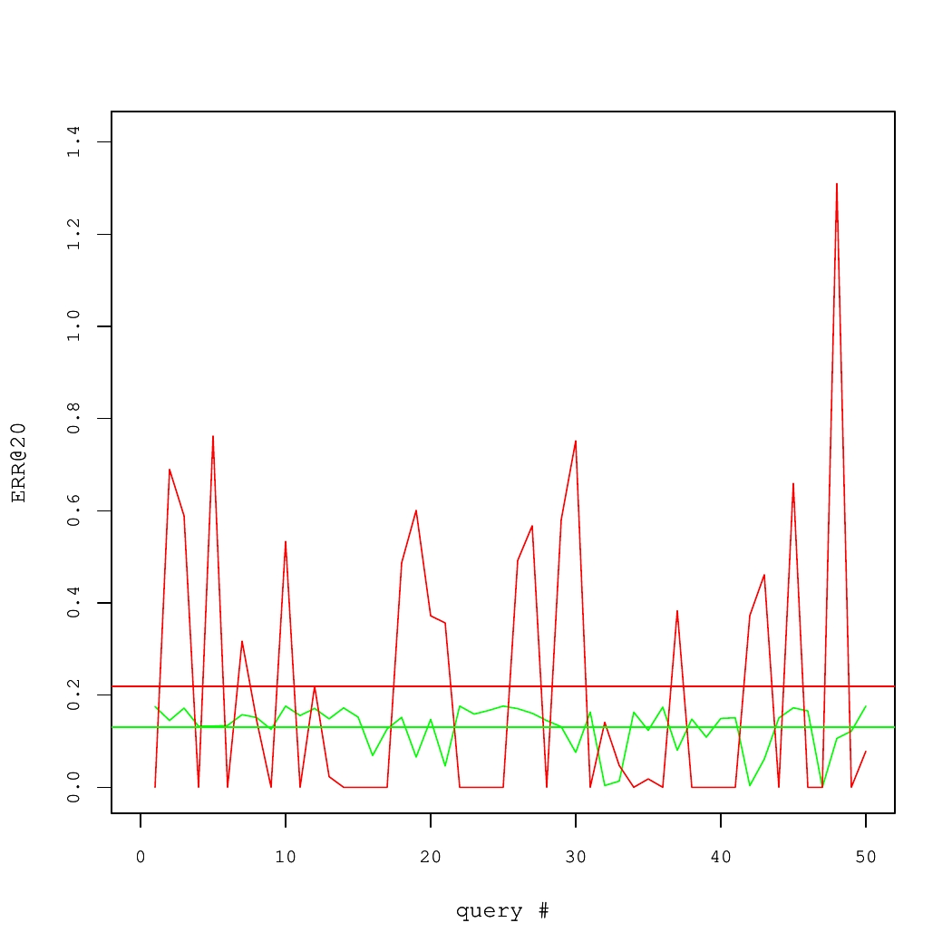
Consider a concrete example of two Information Retrieval (IR) systems, each of which answered 50 queries. The quality of results for each query was measured using a performance metric called the Expected Reciprocal Rank (ERR@20). These numbers are shown in Fig. 1, where average systems' performance values are denoted by horizontal lines.
On average, the red system is better than the green one. Yet, there is high variance. In fact, to produce the Fig. 1, we took query-specific performance scores from one real system and applied an additive zero-centered random noise to generate the other system. If there were sufficiently many queries, this noise would largely cancel out. But for the small set of queries, it is likely that the average performance of two systems would differ.
Fig 1. Performance of two IR systems.
Statistical testing is a standard approach to detect such situations.
Rather than taking average query level values of ERR@20 at their face value, we suppose that there is the sampling uncertainty obfuscating the ground truth about systems' performance. If we make certain assumptions about the nature of randomness (e.g., assume that the noise is normal and i.i.d.), it is possible to determine the likelihood that observed differences are due to chance. In the frequentist inference, this likelihood is represented by a p-value.
The p-value is a probability to obtain an average difference in performance at least as large as the observed one, when truly there is no difference in average systems' performance, or, using the statistical jargon, under the null hypothesis. Under the null hypothesis, a p-value is an instantiation of the uniform random variable between 0 and 1. Suppose that differences in systems' performance corresponding to p-values larger than 0.05 are not considered statistically significant and, thus, ignored. Then, the false positive rate is controlled at 5% level. That is, in only 5% of all cases when the systems are equivalent in the long run, we would erroneously conclude that the systems are different. We would reiterate that in the in frequentist paradigm, the p-value is not necessarily an indicator of how well experimental data support our hypothesis. Measuring p-values (and discarding hypotheses where p-values exceed the 5% threshold) is a method to control the rate of false positives.
Fig. 2. Simulated p-values in 100 experiments, where the true null holds in each experiment.
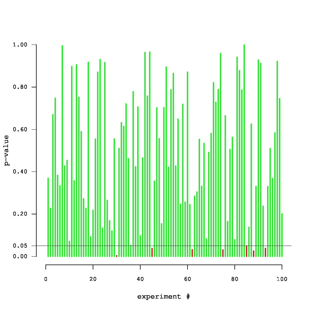
What if the scientist carries out multiple experiments? Consider an example of an unfortunate (but very persistent) researcher, who came up with 100 new systems that were supposed to improve over a given baseline. Yet, they were, in fact, equivalent to the baseline. Thus, each of the 100 p-values can be thought of as an outcome of a uniform random variable between 0 and 1. A set of p-values that could have been obtained in such an experiment is plotted in Fig. 2. The small p-values, below the threshold level of 0.05, are denoted by red bars. Note that one of these p-values is misleadingly small. In truth, there is no improvement in this series of 100 experiments. Thus, there is a danger in paying too much attention to the magnitude of p-values (rather than simply comparing them against a threshold). The issue of multiple testing is universal. In general, most of our hypotheses are false and we expect to observe statistically significant results (all of which are false discoveries) in approximately 5% of all experiments.
This example is well captured by XKCD.
How do we deal with multiple testing? We can decrease the significance threshold or, alternatively, inflate the p-values obtained in the experiments. This process is called an adjustment/correction for multiple testing. The classic correction method is the Bonferroni procedure, where all p-values are multiplied by the number of experiments. Clearly, if the probability of observing a false positive in one experiment is upper bounded by 0.05/100, then the probability that the whole family of 100 experiments contains at least one false positive is upper bounded by 0.05 (due to the union bound).
There are both philosophical and technical aspects of correcting for multiplicity in testing. The philosophical side is controversial. If we adjust p-values in sufficiently many experiments, very few results would be significant! In fact, this observation was verified in the context of TREC experiments (Tague-Sutcliffe, Jean, and James Blustein. 1995, A statistical analysis of the TREC-3 data; Benjamin Carterette, 2012, Multiple testing in statistical analysis of systems-based information retrieval experiments ). But should we really be concerned about joint statistical significance (i.e., significance after we adjust for multiple testing) of our results in the context of the results obtained by other IR researchers? If we have to implement only our own methods, rather than methods created by other people, it is probably sufficient to control the false positive rate only in our own experiments.
We focus on the technical aspects of making adjustments for multiplicity in a single series of experiments. The Bonferroni correction is considered to be overly conservative, especially when there are correlations in data. In an extreme case, if we repeat the same experiment 100 times (i.e., outcomes are perfectly correlated), the Bonferroni correction leads to multiplying each p-value by 100. It is known, however, that we are testing the same method and it is, therefore, sufficient to consider a p-value obtained in (any) single test. The closed testing procedure is a less conservative method that may take correlations into account. It requires testing all possible combinations of hypotheses. This is overly expensive, because the number of combinations is exponential in the number of tested methods. Fortunately, there are approximations to the closed testing procedure, such as the MaxT test, that can also be used.
We carried out an experimental evaluation, which aimed to answer the following questions:
- Is the MaxT a good approximation of the closed testing (in IR experiments)?
- How conservative are multiple comparisons adjustments in the context of a small-scale confirmatory IR experiment?
A description of the experimental setup, including technical details, can be found in our paper (Boytsov, L., Belova, A., Westfall, P. 2013. Deciding on an Adjustment for Multiplicity in IR Experiments. In proceedings of SIGIR 2013.). A brief overview can be found in the presentation slides. Here, we only give a quick summary of results.
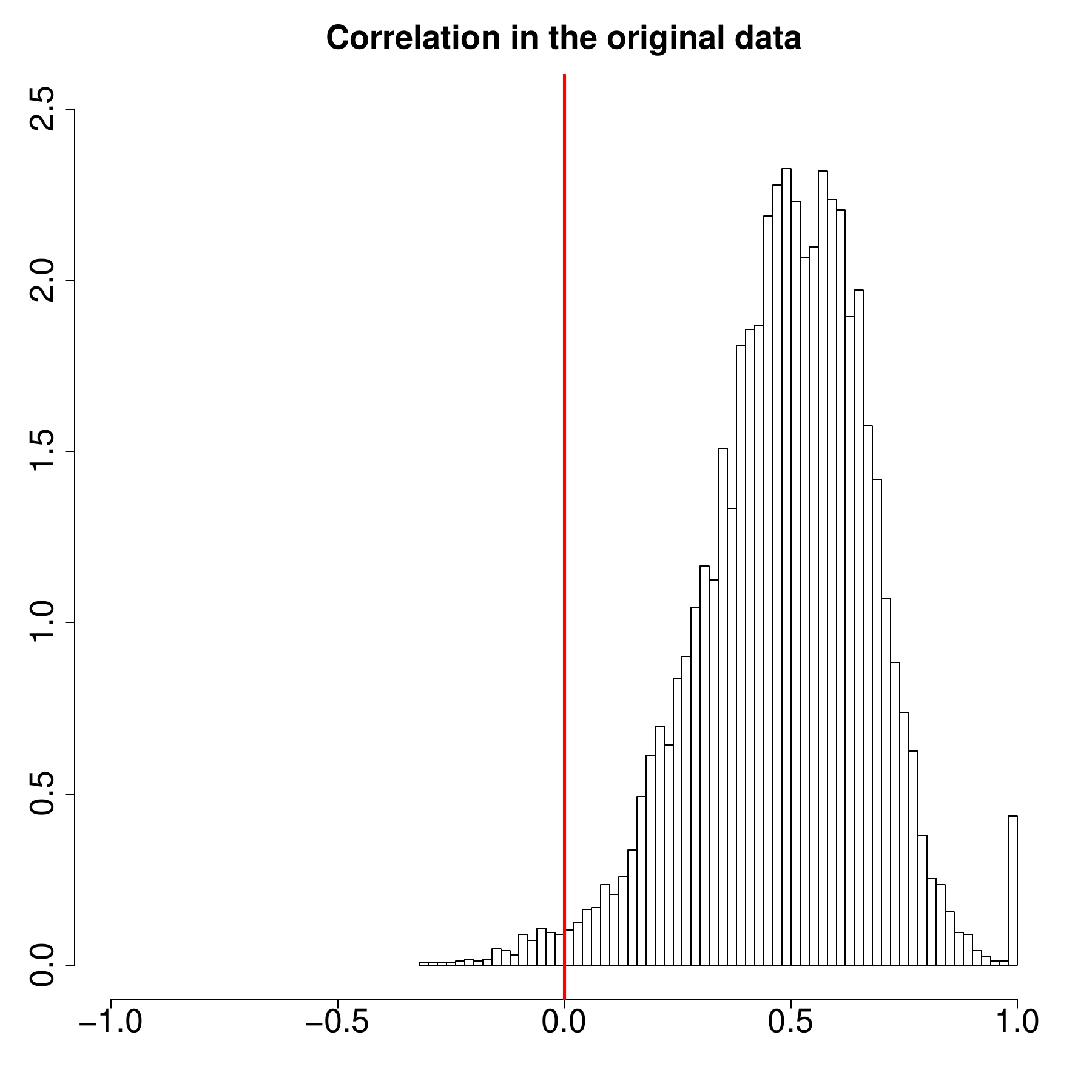
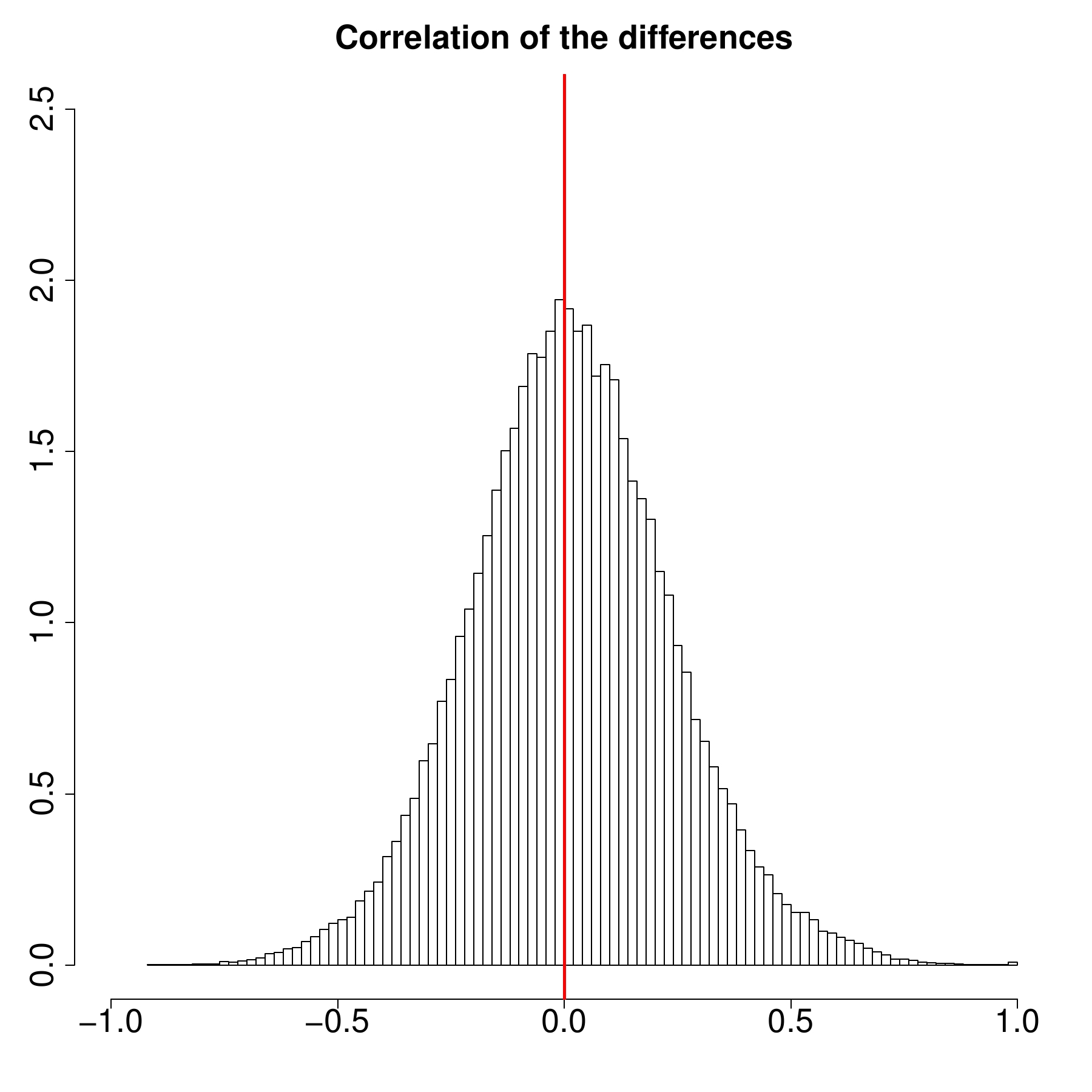
First, in our experiments, the p-values obtained from the MaxT permutation test were almost identical to those obtained from the closed testing procedure. A modification of the Bonferroni adjustment (namely, the Holm-Bonferroni correction) tended to produce larger p-values, but this did not result in the Bonferroni-type correction being much more conservative. This is a puzzling discovery, because performance scores of IR systems (such as ERR@20) substantially correlate with each other (see Fig 3, the panel on the left). In that, both the MaxT permutation test and the closed testing procedure should have outperformed the correlation-agnostic Holm-Bonferroni correction. One possible explanation is that our statistical tests operate essentially on differences in performance scores (rather than scores themselves). It turns out, that there
are fewer strong correlations in performance score differences (see Fig. 3, the panel on the right).
We also carried out a simulation study, in which we measured performance of several systems. Approximately half of our systems were almost identical to the baseline with remaining systems being different. We employed four statistical tests to detect the differences using query sets of different sizes. One of the tests did not involve adjustments for multiplicity. Using average performance values computed for a large set of queries (having 30 thousand elements), we could tell which outcomes of significance testing represented true differences and which were false discoveries. Thus, we were able to compute the number of false positives and false negatives. Note that the fraction of false positives was computed as a fraction of experimental series that contained at least one false positive result. This is called the family-wise error rate.
Table 1. Simulation results for the TREC-like systems. Percentages of false negatives/positives
|
|
|
|
50 |
100 |
400 |
1600 |
6400 |
| Unadjusted test |
85.7/14.4 |
80.8/11.6 |
53.9/10.0 |
25.9/15.4 |
2.5/17.0 |
| Closed test |
92.9/0.0 |
88.8/0.2 |
69.5/1.7 |
36.6/3.1 |
5.2/6.8 |
| MaxT |
93.9/0.0 |
91.8/0.2 |
68.0/1.2 |
35.7/3.0 |
6.3/6.6 |
| Holm-Bonferroni |
94.9/2.0 |
92.5/1.8 |
69.6/2.6 |
37.0/3.2 |
6.5/6.2 |
|
Format: the percentage of false negatives (blue)/false positives (red)
|
|
According to the simulation results in Table 1, if the number of queries is small, the unadjusted test detects around 15% of all true differences (85% false negative rate) . This is twice as many as the number of true differences detected by the tests that adjust p-values for multiple testing. One may conclude that adjustments for multiplicity work poorly and "kill" a lot of significant results. In our opinion, none of the tests performs well, because they discover only a small fraction of all true differences. As the number of queries increases, the differences in the number of detected results between the unadjusted and adjusted tests decrease. For 6400 queries, every test has enough power to detect almost all true differences. Yet, the unadjusted test has a much higher rate of false positives (a higher family-wise error).
Conclusions
We would recommend a wider adoption of adjustments for multiple testing. Detection rates can be good, especially with large query samples. Yet, an important research question is whether we can use correlation structure more effectively.
We make our software available on-line.
Note that it can compute unadjusted p-values as well p-values adjusted for multiple testing. The implementation is efficient (it is written in C++) and accepts data in the form of a performance-score matrix. Thus, it can be applied to other domains, such as classification. We also do provide scripts that can convert the output of TREC evaluation utlities trec_eval and gdeval to the matrix format.
This post was co-authored with Anna Belova
The problem with the previous version of Intel's library benchmark
Submitted by srchvrs on Mon, 04/15/2013 - 01:42
This short post is an update for the previous blog entry. Most likely,
the Intel compiler does not produce the code that is 100x faster, at least, not under normal circumstances. The updated benchmark is posted on the GitHub. Note that the explanation below is just my guess, I will be happy to hear an alternative version.
It looks like the Intel compiler is super-clever and can dynamically adjust accuracy of computation. Consider the following code:
float sum = 0; for (int j = 0; j < rep; ++j) { for (int i = 0; i < N*4; i+=4) { sum += exp(data[i]); sum += exp(data[i+1]); sum += exp(data[i+2]); sum += exp(data[i+3]); } }
Here the sum becomes huge very quickly. Thus, the result of calling exp becomes very small compared to sum. It appears to me that the code built with the Intel compiler does detect this situation. Probably, at run-time. After this happens, the function exp is computed using a very low-accuracy algorithm or not computed at all. As a result, when I ran this benchmark on a pre-historic Intel Core Duo 2GHz, I was still able to crunch billions of exp per second, which was clearly impossible. Consider now the following, updated, benchmark code:
float sum = 0; for (int j = 0; j < rep; ++j) { for (int i = 0; i < N*4; i+=4) { sum += exp(data[i]); sum += exp(data[i+1]); sum += exp(data[i+2]); sum += exp(data[i+3]); } sum /= float(N*4); // Don't allow sum become huge! }
Note line 9. It prevents sum from becoming huge. Now, we are getting more reasonable performance figures. In particular, for single-precision values, i.e., floats,
the Intel compiler produces a code that is only 10x faster compared to code produced by the GNU compiler. It is a large difference, but it is probably due to using SIMD
extensions for Intel.
Pages

|
|
 |
|
|
 |
 |
 |
|
|
|