 |
|
|
|
|
 |
 |
 |
|
|
|
Submitted by srchvrs on Thu, 03/28/2024 - 22:41
Attention folks working on LONG-document ranking & retrieval! We found evidence of a very serious issue in existing long-document collections, most importantly MS MARCO Documents. It can potentially affect all papers comparing different architectures for long document ranking.
Do not get us wrong: We love MS MARCO: It has been a fantastic resource that spearheaded research on ranking and retrieval models. In our work we use MS MARCO both directly as well as its derivative form: MS MARCO FarRelevant.
Yet MS MARCO (and similar collections) can have substantial positional biases which not only "mask" differences among existing models, but also prevent MS MARCO trained models from performing well on some other collections.
This is not a modest degradation where performance drops roughly to BM25 level (as we observed, e.g., in our prior evaluation).. It can be a dramatic drop in accuracy down to the random baseline level.
We found a substantial positional bias of relevant information in standard IR collections, which include MS MARCO Documents and Robust04. However, judging from other paper results a lot of other collections are affected.
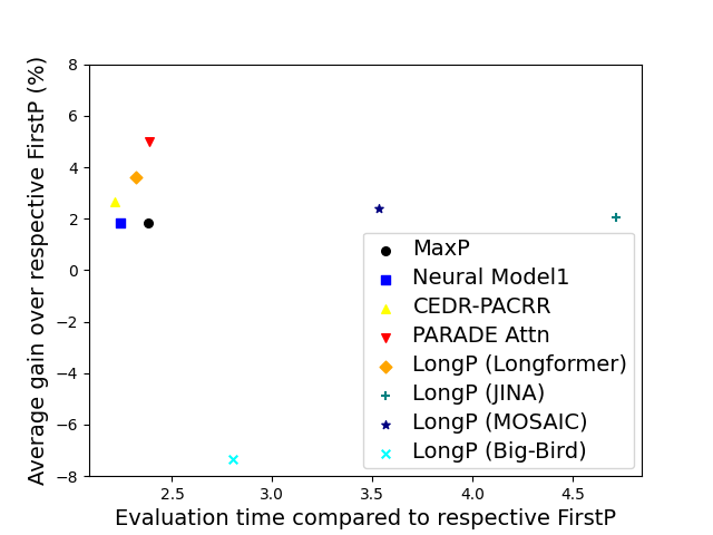
Because relevant info tends to be in the beginning of a doc we often do not need a special long-context model to do well in ranking and retrieval. The so-called FirstP model (truncation to < 512 tokens) can do well (see the picture, we do not plot FirstP explicitly, but all the numbers are relative to FirstP efficiency or accuracy):
So how do we prove positional bias is real? There is no definitive evidence, but we provide several evidence pieces. In doing so we introduce a NEW synthetic collection MS MARCO Far Relevant which does not have relevant passages in the beginning.
- On MS MARCO we trained 20+ rank models (including two FlashAttention-based models) and observed all of them to barely beat FirstP (in rare cases models underperformed FirstP);.
- We analyzed positions of relevant passages and found these to be skewed to the beginning;
- We 0-shot tested & then fine-tuned models on MS MARCO Far Relevant.
Unlike standard collections where we observed both little benefit from incorporating longer contexts & limited variability in model performance (within a few %), experiments on MS MARCO FarRelevant uncovered dramatic differences among models.
-
To begin with, FirstP models performed roughly at the random-baseline level in both 0-shot and fine-tuning scenarios (see the picture below).
-
Second, simple aggregation models including MaxP and PARADE Attention had good zero-shot accuracy, but benefited little from fine-tuning.
-
In contrast, most other models had poor 0-shot performance (roughly at a random baseline level), but outstripped MaxP by as much as 13-28% after fine-tuning. Check out the lines connecting markers in left and right columns:
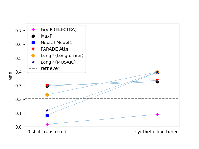
Best models? PARADE models were the best and markedly outperformed FlashAttention-based models, Longformer as well as chunk-and-aggregate approaches. PARADE Attention performed best on standard collection (in most cases) and in the zero-shot transfer model on MS MARCO FarRelevant. However, among fine-tuned models on MS MARCO Far Relevant, the best was PARADE Transformer (with a randomly initialized aggregator model).
This paper is an upgrade of 2021 preprint enabled by a great collaborator David Akinpelu as well as by the team of former CMU (MCDS) students. David, specifically, did a ton of work including implementation of recent baselines.
Paper link.
Code/Data link
Submitted by srchvrs on Sun, 07/26/2026 - 14:11
I have some thoughts related to the recent craze to automate everything with agentic skills. On a plus side, I think it can be very useful when done correctly. On the negative side, it is often done incorrectly and only adds more technical debt. Instead of solving systemic issues first, people are just slapping an AI band-aid in the hope to stop a gushing artery.
Using an agent (and essentially an LLM) as the primary orchestrator for deterministic workflows sacrifices many of the properties that decades of good software engineering have optimized for. We lose predictability, reproducibility, testability, debuggability, and the ability to reason formally about system behavior. More subtly, we often sacrifice encapsulation: instead of components exposing explicit, versioned interfaces, the LLM needs to understand implementation details and prompt conventions. This increases coupling between components, makes the overall system less coherent, and turns what should be local implementation changes into workflow-wide prompt adjustments. One should not forget that natural language is imprecise and ambiguous so it is in principle impossible to define complex workflows accurately.
Humans often lack understanding of how the agent interoperates with different components and it is hard to debug or predict how LLM will behave. For workflows where an execution sequence can be well defined (which includes quite a few workflows), the agent's role should be much narrower. It should primarily act as a thin interface layer: gather user intent, fill slots, perform lightweight validation, and invoke a well-defined sequence of deterministic scripts or services. The workflow itself should be explicit, documented, version-controlled, and independently executable. Mixing code-snippets and natural language commands in a single SKILLS.md file feels like an engineering antipattern. It tightly couples deterministic scripts with a non-deterministic sequence of steps defined by the agents and makes debugging extremely difficult. What makes debugging difficult is not just the nondeterminism. It's that the control flow becomes implicit rather than explicit.
Agent-based orchestration has an important operational requirement. If something goes wrong (whether due to an LLM hallucination, a provider outage, a rate limit from Codex or Claude Code, or simply an unexpected edge case) a human engineer should be able to resume or rerun the workflow manually by invoking the same documented scripts. The system should remain inspectable and recoverable because the deterministic backbone exists independently of the agent. In my experience, this requirement is frequently overlooked.
Agents still have valuable roles outside the critical execution path where their use is more flexible. They can assist with debugging failures, investigating unexpected outcomes, suggesting fixes, summarizing logs, or helping operators understand complex system state. In those cases, occasional mistakes are acceptable because a human is already in the loop. Moreover, when something goes wrong, it is better to obtain a quick (though possibly not 100% precise) assessment of the situation rather than waste days to obtain a correct one. But the production workflow itself should remain deterministic whenever the problem domain permits it.
Submitted by srchvrs on Mon, 03/09/2026 - 14:41
For the last seven years, I kept re-implementing the same pattern: A parallel map loop that divides the work among several processes or threads..
My very first attempts were built on Python’s standard tools, e.g., multiprocessing.map, and I later explored pqdm (the “Parallel TQDM” library) to simplify the code (as well as to visualize progress on long-running loops) when workers were stateless. Those solutions did work but always felt incomplete and required repeated boilerplate. Much later did I explore tools like Dask and Ray (see examples in the end of the post) and found that, for this specific pattern, they still required a lot of complexity and infrastructure for something that should be simple: A simple, streaming, stateful, parallel map loop with accurate progress tracking and minimal boilerplate — that actually works everywhere.
In 2024, I finally distilled the pattern into a tiny library: mtasklite.
Below is the motivation, the flaws of existing approaches, and what makes mtasklite unique.
Common Pain Points with Existing Tools
Even for simple parallel loops, many libraries fall short:
1. Stateful workers with flexible initialization
Most map APIs assume stateless functions. When workers must load models or context before processing, solutions become awkward or require elaborate hacks.
2. True streaming input/output
Many frameworks materialize outputs in bulk rather than yielding results as soon as they are ready. This breaks bounded-memory pipelines.
3. Size-aware streaming for progress tracking for limited-size input/output
Tools that process fixed-size input arrays often fail to expose an output with a usable len(...). Without a known length, progress bars like tqdm can’t estimate remaining time.
4. Notebook compatibility
Some parallel tools (e.g., Ray actors, certain ways of using multiprocessing) behave unpredictably in Jupyter/IPython environments.
5. Boilerplate and cognitive overhead
Great libraries like Dask and Ray are powerful, but for a simple map pattern they introduce clusters, schedulers, plugins, actors, futures, and daemons (see examples in the end of the post).
6. Lightweight API
Many real workloads don’t need a full distributed system — just a clean, streaming, parallel map loop.
A more detailed discussion of these limitations follows later.
What Makes mtasklite Different
Minimal Boilerplate
You don’t need:
- Clusters or schedulers
- Actors or plugins
- Futures or object references, which need to be checked for completion
- Background daemons or services
Stateful Workers with Flexible Initialization
Workers can:
- Initialize once with stateful setup
- Receive per-worker init arguments
- Maintain local state across tasks
This is essential for real workloads — model loading, database connections, tokenizers, GPU context, etc.
True Streaming Input + Output
mtasklite works with:
- Any input iterator
- True streaming of results
⟶ Outputs appear as soon as they’re ready
⟶ Memory stays bounded (unless requested)
⟶ No buffering of the entire input and output set
This is crucial for real world pipelines that process huge datasets.
Size-Aware Output for Progress Bars
When the input iterator has a known length, the mtasklite output iterator provides a length function as well. This enables easy and accurate progress bars (tqdm, etc.).
Works Everywhere
No matter the environment:
- Jupyter Notebooks
- Python REPL
- Scripts
- Interactive environments
mtasklite avoids features that frequently misbehave in notebooks or interactive shells.
Lightweight and Elegant API
The API stays close to familiar Python map semantics:
for out in parallel_map(f, xs): ...
Easy Migration from pqdm
If you’re already a pqdm user — the “Parallel TQDM” library built on concurrent.futures + tqdm — switching to mtasklite is very easy. The API is nearly 100% compatible, and there’s a dedicated migration guide describing a couple of tiny but necessary differences.
That means you can enjoy:
- Per-worker initialization
- True streaming output
- Sized iterators for progress bars
- Notebook-friendly behavior
…without rewriting your existing loops.
A Motivating Example
Below is a (somewhat contrived) example of a stateful, class-based, worker that computes a square root. It is implemented as a regular class with the constructor and a __call__ function with the only nuance: It is decorated using the @delayed_init decorator. This decorator "wraps" the actual object inside a shell object, which only memorizes object's initialization parameters. An actual instantiation is delayed till a worker process (or thread) starts.
from mtasklite import delayed_init from mtasklite.processes import pqdm @delayed_init class Square: def __init__(self, worker_id): print(f"Initializing worker {worker_id}") def __call__(self, x): return x * x inputs = [1, 2, 3, 4, 5] with pqdm(inputs, [Square(0), Square(1), Square(2), Square(3)]) as out: for y in out: print(y)
This provides:
- Stateful worker initialization
- Streaming output
- Sized iterator compatible with progress bars
- Bounded memory
- Works in notebooks and scripts
- No external infrastructure
Why Other Tools Did Not Fit
Below is a concise explanation of why other popular tools don’t satisfy this pattern without complexity.
multiprocessing + tqdm
Using multiprocessing and tqdm together requires a lot of repetition and manual work:
- Worker init routines are limited
- Integrating with progress bars often requires imap/imap_unordered patterns
- You must manage iterator lengths manually to drive tqdm correctly
- Behavior can be unpredictable in notebooks
Yes, you can piece together something yourself — but you end up rewriting the same wrapper logic repeatedly. Below is an example of how cumbersome it is:
from tqdm.auto import tqdm from multiprocessing import Pool def init_worker(proc_id): global WORKER_ID WORKER_ID = proc_id print(f"[Worker init] ID = {WORKER_ID}") def worker_task(a): # Use global WORKER_ID if needed return a * a if __name__ == "__main__": proc_ids = [0,1,2,3] input_vals = list(range(20)) chunksize=1 result = [] with Pool(processes=len(proc_ids), initializer=init_worker, initargs=(proc_ids.pop(0),)) as pool: # map is a blocking call that return the result only when all input is processed #for ret_val in tqdm(pool.map(worker_task, input_vals, chunksize)): for ret_val in tqdm(pool.imap(worker_task, input_vals, chunksize)): result.append(ret_val) print(result)
Dask
Dask is powerful for distributed computation, but for this pattern it is an overkill (which, again, requires additional boilerplate).Dask excels at DAGs and large dataframes, but doesn’t treat this lightweight map pattern as a first-class use case. In this specific example it was also 10x slower compared to mtasklite (with a 6-core Intel Mac).
from dask.distributed import LocalCluster, Client from tqdm.auto import tqdm class SquareActor: def __init__(self, proc_id): import multiprocess as mp print(f"Initialized process {mp.current_process()} with argument = {proc_id}") self.proc_id = proc_id def compute(self, a): # Method to call for each task return a * a def run_with_square_actors(input_arr, proc_ids): # Start cluster & client via context managers with LocalCluster(n_workers=len(proc_ids), processes=True) as cluster: with Client(cluster) as client: # Create one actor per proc_id actor_futures = [ client.submit(SquareActor, pid, actor=True) for pid in proc_ids ] actors = [f.result() for f in actor_futures] # Dispatch work to actors by calling the method `.compute(...)` results = [] for i, val in enumerate(tqdm(input_arr)): actor = actors[i % len(actors)] # This returns an actor future; .result() waits for execution results.append(actor.compute(val).result()) return results if __name__ == "__main__": input_arr = list(range(20)) proc_ids = [0, 1, 2, 3] result = run_with_square_actors(input_arr, proc_ids) print(result)
Ray
Ray’s actor model solves stateful workers elegantly, but:
- Ray runtime initialization often conflicts with notebooks
- There’s no built-in streaming map API; you write your own loops
- API feels distributed-system-first rather than lightweight
Ray is a powerful platform, but still not “simple map loop first.” It can also be quite heavy-weight (due to start up overhead). In this specific example, it is about 40x slower compared to mtasklite:
#!/usr/bin/env python import ray from collections import deque from tqdm.auto import tqdm ray.init() @ray.remote class Worker: def __init__(self, proc_id): import multiprocess as mp print(f"Initialized worker {proc_id} in process {mp.current_process()}") self.proc_id = proc_id def compute(self, x): return x * x def ray_stateful_stream_map(inputs, proc_ids, worker_qty=8): """ A generator that streams outputs as they complete, using stateful Ray actors with proc_ids. Args: inputs: An iterable of inputs. proc_ids: A list of init args for each actor. worker_qty: Max number of workers """ actors = [Worker.remote(pid) for pid in proc_ids] pending = deque() it = iter(inputs) # Submit initial batch for _ in range(min(worker_qty, len(proc_ids))): try: val = next(it) except StopIteration: break # round-robin actor = actors[len(pending) % len(actors)] pending.append(actor.compute.remote(val)) while pending: # Wait for the next ready future ready, _ = ray.wait(list(pending), num_returns=1) ref = ready[0] pending.remove(ref) yield ray.get(ref) # Submit more work try: val = next(it) actor = actors[len(pending) % len(actors)] pending.append(actor.compute.remote(val)) except StopIteration: pass result = [] for ret_val in tqdm(ray_stateful_stream_map(range(1, 21), proc_ids=[0,1,2,3], worker_qty=8)): result.append(ret_val) print(result)
Conclusion
I did not set out to build another parallelism library — I just kept rewriting this same code for six years:
- Stateful workers with init
- Streaming outputs
- Sized outputs for progress bars
- Minimal boilerplate
- Works everywhere
Once I distilled it into a tiny, composable API, it became clear this pattern deserved its own package.
That package is mtasklite — a tiny, elegant, minimal toolkit for real-world parallel map loops.
GitHub:
https://github.com/searchivarius/py_mtasklite
Submitted by srchvrs on Tue, 08/26/2025 - 19:08
I recently finished, perhaps, my nerdiest computer science paper so far and it was accepted by TMLR: A Curious Case of Remarkable Resilience to Gradient Attacks via Fully Convolutional and Differentiable Front End with a Skip Connection. This work was done while I was at the Bosch Center of AI (outside my main employment at Amazon), but I was so busy that I had little time to put it in writing. I submitted the first draft only last year, and it required a major revision, which I was able to finish only in July. It is not a particularly practical paper—I accidentally discovered an interesting and puzzling phenomenon and decided to document it (with a help of my co-authors).
The following AI-generated summary, I believe, provides an accurate description of our work:
The paper presents a fascinating case study on how a seemingly innocuous modification to a neural network can drastically alter its perceived robustness against adversarial attacks. I accidentally discovered a simple yet surprisingly effective technique: prepending a frozen backbone classifier with a differentiable and fully convolutional "front end" model containing a skip connection. This composite model, when trained briefly with a small learning rate, exhibits remarkable resistance to gradient-based adversarial attacks, including those within the popular AutoAttack framework (APGD, FAB-T).
Here's a breakdown of the paper's core elements, methodology, and findings in more detail:
1. The Curious Phenomenon:
-
We observed that adding a differentiable front end to a classifier significantly boosted its apparent robustness to adversarial attacks, particularly gradient-based ones.
-
This robustness occurred without significantly sacrificing clean accuracy (accuracy on non-adversarial, original data).
-
The effect was reproducible across different datasets (CIFAR10, CIFAR100, ImageNet) and various backbone models (ResNet, Wide ResNet, Vision Transformers).
-
The training recipe for the front end (small learning rate, short training duration) was stable and reliable.
2. The Front End Architecture (DnCNN):
-
The front end used is based on DnCNN (Denoising Convolutional Neural Network), a fully convolutional architecture with skip connections.
-
Skip connections are crucial for training deep networks. They help the gradient flow more smoothly during backpropagation, preventing vanishing gradients.
-
DnCNN is differentiable. Unlike some adversarial defense strategies that rely on non-differentiable components (like JPEG compression) to disrupt gradient-based attacks, DnCNN allows gradients to be computed throughout the entire network.
-
We argue that the success of this method is especially surprising because the use of a skip connection is actually expected to improve gradient flow, not to mask gradients.
Submitted by srchvrs on Thu, 08/18/2022 - 00:37
The Hugging Face Accelerate library provides a convenient set of primitives for distributed training on multiple devices including GPUs, TPUs, and hybrid CPU-GPU systems (via Deepspeed). Despite convenience, there is one drawback: Only a synchronous SGD is supported. After gradients are computed (possibly in a series of accumulation steps), they are synchronized among devices and the model is updated. However, gradient synchronization is costly and it is particularly costly for consumer-grade GPUs, which are connected via PCI Express.
For example, if you have a 4-GPU server with a 16-lane PCI express v3, your synchronization capacity seems to be limited to 16 GB per second [1]. Without fast GPU interconnect, gradient synchronization requires transferring of each model weights to CPU memory with subsequent transfers to three other GPUs. This would be 16 transfers in total. If PCI express is fully bidirectional (which seems to be the case), this can be done a bit more efficiently (with 12 transfers) [2]. According to my back-of-the-envelope estimation gradient synchronization can take about the same time as training itself [3]! Thus, there will be little (if any) benefit of multi-GPU training.
Without further speculation, let us carry out an actual experiment (a simple end-to-end script to do so is available). I train a BERT large model for a QA task using two subsets of SQuAD v1 dataset (4K and 40K samples) using either one or four GPUs. Each experiment was repeated three times using different seeds. All results (timings and accuracy values) are provided.
In the multi-GPU setting, I use either a standard fully synchronous SGD or an SGD that synchronizes gradients every K batches. Note that the non-synchronous variant is hacky proof-of-concept (see the diff below), which likely does not synchronize all gradients (and it may be better to synchronize just model weights instead), but it still works pretty well.
For the fully synchronous SGD, each experiment is carried out using a varying number of gradient accumulation steps. If I understand the code of Accelerate correctly, the more accumulation steps we make, the less frequent is synchronization of gradients, so having more accumulation steps should permit more efficient training (but the effective batch size increases).
# of training
samples |
Single-GPU |
Multi-GPU (four GPUs)
fully synchronous SGD
varying # of gradient accumulation steps |
Multi-GPU (four GPUs)
k-batch synchronous SGD
varying # of gradient synchronization steps |
|---|
|
|
1 |
2 |
4 |
8 |
16 |
1 |
2 |
4 |
8 |
16 |
| 4000 |
f1=79.3 |
f1=77.8 2.6x |
f1=74.7 2.7x |
f1=70.6 2.7x |
f1=54.8 2.9x |
f1=15.9 3.1x |
f1=77.4 2.6x |
f1=74.5 2.9x |
f1=71.9 3.3x |
f1=72.8 3.5x |
f1=74.2 3.6x |
| 40000 |
f1=89.2 |
f1=88.6 2.4x |
f1=88.2 2.5x |
f1=87.5 2.6x |
f1=86.7 2.6x |
f1=84.4 2.6x |
f1=88.8 2.4x |
f1=87.2 2.8x |
f1=87.3 3.2x |
f1=87.4 3.4x |
f1=87.3 3.6x |
The result table shows both the accuracy (F1-score) and the speed up with respect to a single-GPU training. First, we can see that using a small training set results in lower F1-scores (which is, of course, totally expected). Second, there is a difference between single-GPU training and fully-synchronous SGD, which is likely due to increase in the effective batch size (when all four GPUs are used). For the larger 40K training set the degradation is quite small. In any case, we use F1-score for the fully synchronous multi-GPU training as a reference point for the perfect accuracy score.
When we use the fully synchronous SGD, the increase of the number of gradient accumulation steps leads only to a modest speed up, which does not exceed 2.6x for the larger 40K set. At the same time, there is a 5% decrease in F1-score on the larger set and a catastrophic 3x reduction for the 4K set! I verified this dramatic loss cannot be easily fixed by changing the learning rate (at least I did not find good ones).
In contrast, for the non-synchronous SGD, there is a much smaller loss in F1-score when the synchronization interval increases. For the larger 40K training set, synchronizing one out of 16 batches leads to only 1.7% loss in F1-score. In that, the speed-up can be as high as 3.6x. Thus, our POC implementation of the non-synchronous SGD, which as I mentioned earlier is likely to be slightly deficient, is (nearly) always (often much) better than the current fully synchronous SGD implemented in Accelerator.
To reiterate, Accelerator supports only the synchronous SGD, which requires a costly synchronization for every batch. This is not an efficient setup for servers without a fast interconnect. A common "folklore" approach (sorry, I do not have a precise citation) is to relax this requirement and synchronize model weights (or accumulated gradients) every K>1 batches [4]. This is the approach I implemented in FlexNeuART and BCAI ART. It would be great to see this approach implemented in Accelerator as well (or directly in Pytorch).
Notes:
[1] Interconnect information can be obtained via nvidia-smi -a.
[2] I think fewer than 12 bidirectional transfers would be impossible. Optimistically we can assume updated weights/gradients are already in the CPU memory, then each model weights/gradients need to be delivered to three other GPUs. In practice, 12 transfers are actually possible by moving data from one GPU's memory to CPU memory and immediately to another GPU's memory. After four such bi-directional transfers all data would be in the CPU memory. Thus, to finalize the synchronization process we would need only eight additional unidirectional (CPU-to-GPU) transfers.
[3] For a BERT large model (345M parameters) with half-precision gradients each gradient synchronization entails moving about 0.67 GB of data. As mentioned above, synchronization requires 12 bidirectional transfers for a total of 12 x 0.67 = 8GB of data. Thus, we can synchronize only twice per second. At the same time, when using a single GPU the training speed of BERT large on SQuAD QA data is three iteration/batches per second. Thus, gradient synchronization could take about the same time as training itself! My back-of-the-envelope calculations can be a bit off (due to some factors that I do not take into account), but they should be roughly in the ballpark.
[4] The parameter value K needs to be tuned. However, I find that its choice does not affect accuracy much unless K becomes too large. Thus it is safe to increase K until we achieve a speed-up close to the maximal possible one (e.g., 3.5x speed up with four GPUs). In my (admittedly limited) experience, this never led to noticeable loss in accuracy and sometimes it slightly improved results (apparently because non-synchronous SGD is a form of regularization).
A partial diff. between the original (fully-synchronous) and K-batch synchronous trainer (this is just a POC version, which is not fully correct):
@@ -760,6 +767,9 @@ num_training_steps=args.max_train_steps, ) + orig_model = model + orig_optimizer = optimizer + # Prepare everything with our `accelerator`. model, optimizer, train_dataloader, eval_dataloader, lr_scheduler = accelerator.prepare( model, optimizer, train_dataloader, eval_dataloader, lr_scheduler @@ -834,6 +845,7 @@ for epoch in range(starting_epoch, args.num_train_epochs): model.train() + orig_model.train() if args.with_tracking: total_loss = 0 for step, batch in enumerate(train_dataloader): @@ -842,17 +854,27 @@ if resume_step is not None and step < resume_step: completed_steps += 1 continue - outputs = model(**batch) + grad_sync = (step % args.no_sync_steps == 0) or (step == len(train_dataloader) - 1) + if grad_sync: + curr_model = model + curr_optimizer = optimizer + else: + curr_model = orig_model + curr_optimizer = orig_optimizer + outputs = curr_model(**batch) loss = outputs.loss # We keep track of the loss at each epoch if args.with_tracking: total_loss += loss.detach().float() loss = loss / args.gradient_accumulation_steps - accelerator.backward(loss) + if grad_sync: + accelerator.backward(loss) + else: + loss.backward() if step % args.gradient_accumulation_steps == 0 or step == len(train_dataloader) - 1: - optimizer.step() + curr_optimizer.step() lr_scheduler.step() - optimizer.zero_grad() + curr_optimizer.zero_grad() progress_bar.update(1) completed_steps += 1 @@ -896,6 +918,7 @@ all_end_logits = [] model.eval() + orig_model.eval() for step, batch in enumerate(eval_dataloader): with torch.no_grad():
Pages

|
|
 |
|
|
 |
 |
 |
|
|
|