The job of scientists is to explain "... life, the universe, and everything". The scientific hunt starts with collecting limited evidence and making guesses about relationships among observed data. These guesses, also known as hypotheses, are based on little data and require verification.
According to the Oxford Dictionary, systematic observation, testing and modification of hypotheses
is the essence of the scientific method.
Our minds are quite inventive in producing theories, but testing theories is expensive and time consuming. To test a hypothesis, one needs to measure the outcome under different conditions. Measurements are error-prone and there may be several causes of the outcome, some of which are hard to observe, explain, and control.
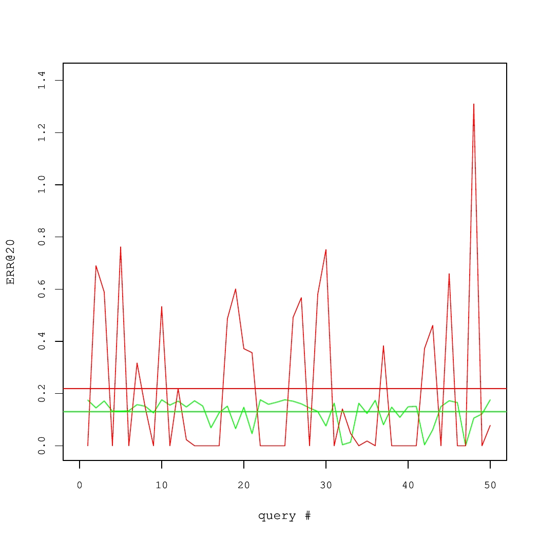
Consider a concrete example of two Information Retrieval (IR) systems, each of which answered 50 queries. The quality of results for each query was measured using a performance metric called the Expected Reciprocal Rank (ERR@20). These numbers are shown in Fig. 1, where average systems' performance values are denoted by horizontal lines.
On average, the red system is better than the green one. Yet, there is high variance. In fact, to produce the Fig. 1, we took query-specific performance scores from one real system and applied an additive zero-centered random noise to generate the other system. If there were sufficiently many queries, this noise would largely cancel out. But for the small set of queries, it is likely that the average performance of two systems would differ.
Fig 1. Performance of two IR systems.
Statistical testing is a standard approach to detect such situations.
Rather than taking average query level values of ERR@20 at their face value, we suppose that there is the sampling uncertainty obfuscating the ground truth about systems' performance. If we make certain assumptions about the nature of randomness (e.g., assume that the noise is normal and i.i.d.), it is possible to determine the likelihood that observed differences are due to chance. In the frequentist inference, this likelihood is represented by a p-value.
The p-value is a probability to obtain an average difference in performance at least as large as the observed one, when truly there is no difference in average systems' performance, or, using the statistical jargon, under the null hypothesis. Under the null hypothesis, a p-value is an instantiation of the uniform random variable between 0 and 1. Suppose that differences in systems' performance corresponding to p-values larger than 0.05 are not considered statistically significant and, thus, ignored. Then, the false positive rate is controlled at 5% level. That is, in only 5% of all cases when the systems are equivalent in the long run, we would erroneously conclude that the systems are different. We would reiterate that in the in frequentist paradigm, the p-value is not necessarily an indicator of how well experimental data support our hypothesis. Measuring p-values (and discarding hypotheses where p-values exceed the 5% threshold) is a method to control the rate of false positives.
Fig. 2. Simulated p-values in 100 experiments, where the true null holds in each experiment.
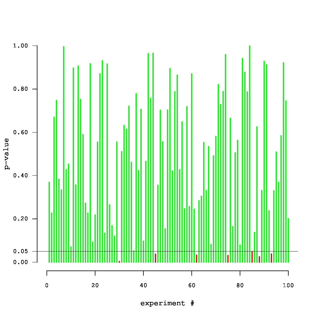
What if the scientist carries out multiple experiments? Consider an example of an unfortunate (but very persistent) researcher, who came up with 100 new systems that were supposed to improve over a given baseline. Yet, they were, in fact, equivalent to the baseline. Thus, each of the 100 p-values can be thought of as an outcome of a uniform random variable between 0 and 1. A set of p-values that could have been obtained in such an experiment is plotted in Fig. 2. The small p-values, below the threshold level of 0.05, are denoted by red bars. Note that one of these p-values is misleadingly small. In truth, there is no improvement in this series of 100 experiments. Thus, there is a danger in paying too much attention to the magnitude of p-values (rather than simply comparing them against a threshold). The issue of multiple testing is universal. In general, most of our hypotheses are false and we expect to observe statistically significant results (all of which are false discoveries) in approximately 5% of all experiments.
This example is well captured by XKCD.
How do we deal with multiple testing? We can decrease the significance threshold or, alternatively, inflate the p-values obtained in the experiments. This process is called an adjustment/correction for multiple testing. The classic correction method is the Bonferroni procedure, where all p-values are multiplied by the number of experiments. Clearly, if the probability of observing a false positive in one experiment is upper bounded by 0.05/100, then the probability that the whole family of 100 experiments contains at least one false positive is upper bounded by 0.05 (due to the union bound).
There are both philosophical and technical aspects of correcting for multiplicity in testing. The philosophical side is controversial. If we adjust p-values in sufficiently many experiments, very few results would be significant! In fact, this observation was verified in the context of TREC experiments (Tague-Sutcliffe, Jean, and James Blustein. 1995, A statistical analysis of the TREC-3 data; Benjamin Carterette, 2012, Multiple testing in statistical analysis of systems-based information retrieval experiments ). But should we really be concerned about joint statistical significance (i.e., significance after we adjust for multiple testing) of our results in the context of the results obtained by other IR researchers? If we have to implement only our own methods, rather than methods created by other people, it is probably sufficient to control the false positive rate only in our own experiments.
We focus on the technical aspects of making adjustments for multiplicity in a single series of experiments. The Bonferroni correction is considered to be overly conservative, especially when there are correlations in data. In an extreme case, if we repeat the same experiment 100 times (i.e., outcomes are perfectly correlated), the Bonferroni correction leads to multiplying each p-value by 100. It is known, however, that we are testing the same method and it is, therefore, sufficient to consider a p-value obtained in (any) single test. The closed testing procedure is a less conservative method that may take correlations into account. It requires testing all possible combinations of hypotheses. This is overly expensive, because the number of combinations is exponential in the number of tested methods. Fortunately, there are approximations to the closed testing procedure, such as the MaxT test, that can also be used.
We carried out an experimental evaluation, which aimed to answer the following questions:
- Is the MaxT a good approximation of the closed testing (in IR experiments)?
- How conservative are multiple comparisons adjustments in the context of a small-scale confirmatory IR experiment?
A description of the experimental setup, including technical details, can be found in our paper (Boytsov, L., Belova, A., Westfall, P. 2013. Deciding on an Adjustment for Multiplicity in IR Experiments. In proceedings of SIGIR 2013.). A brief overview can be found in the presentation slides. Here, we only give a quick summary of results.
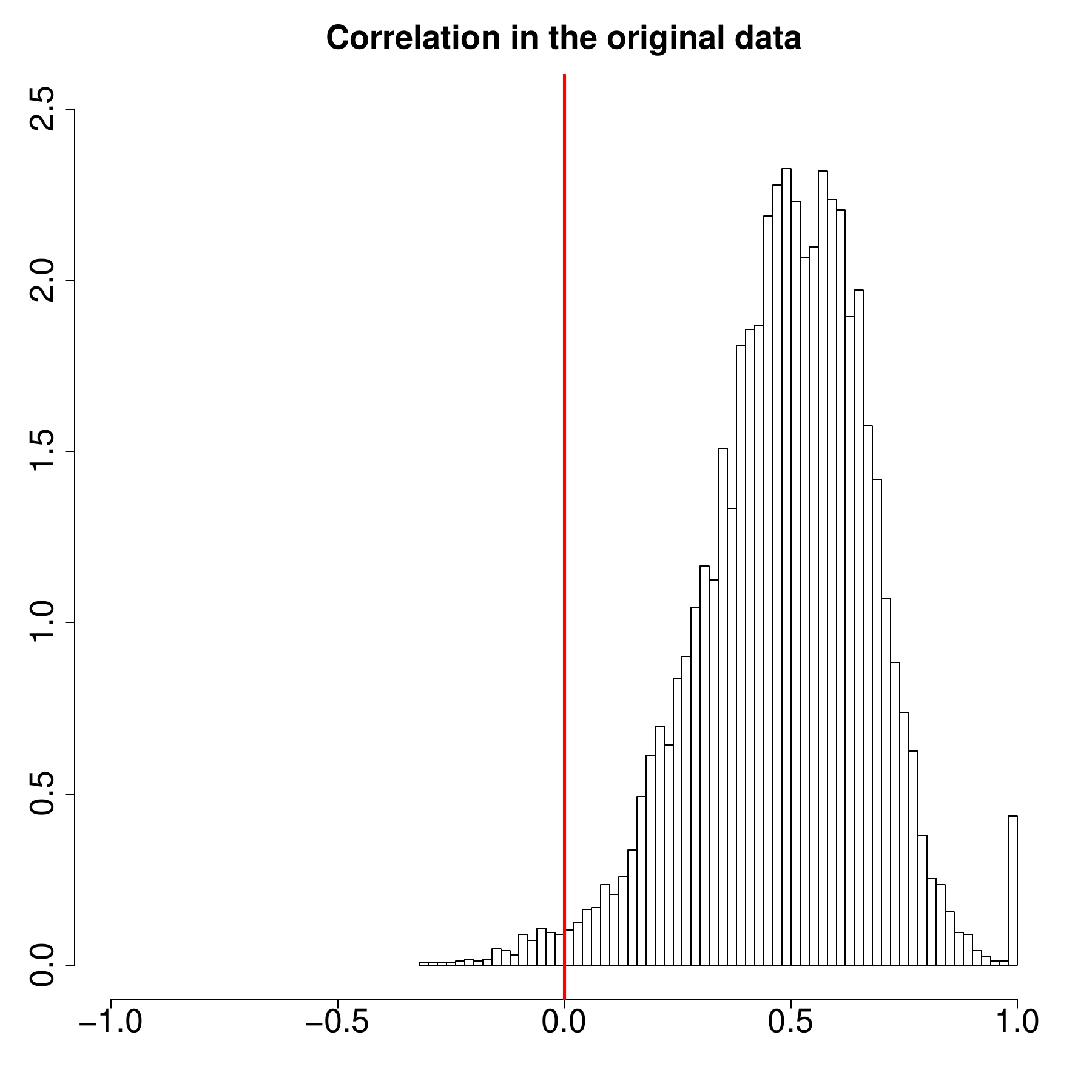
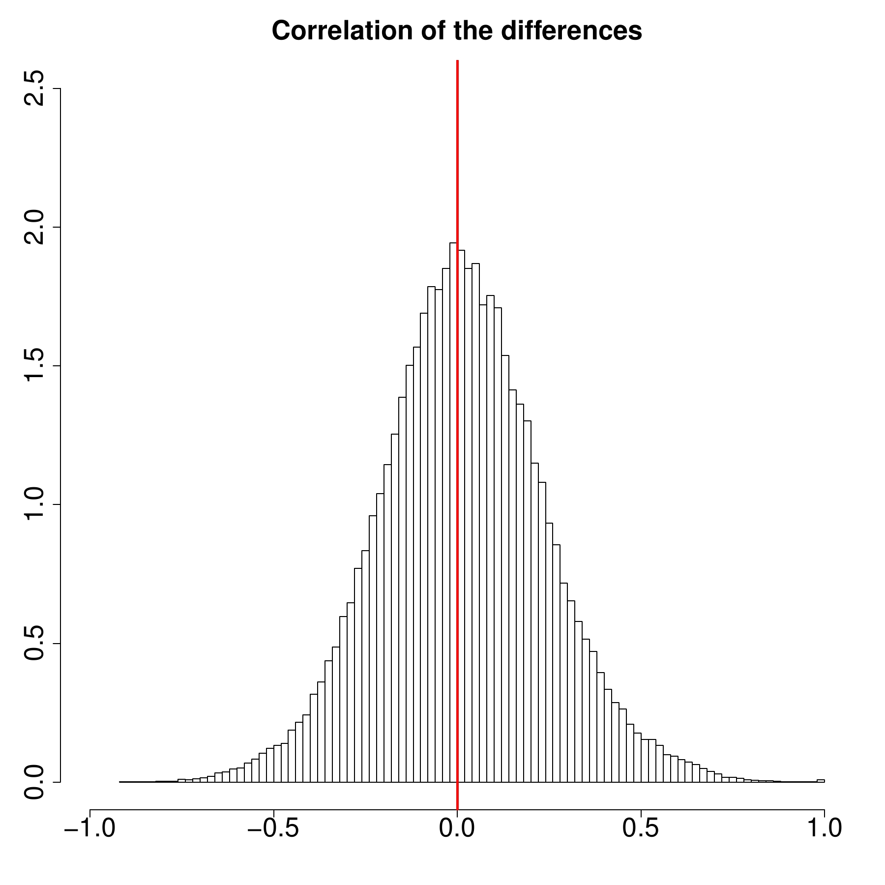
First, in our experiments, the p-values obtained from the MaxT permutation test were almost identical to those obtained from the closed testing procedure. A modification of the Bonferroni adjustment (namely, the Holm-Bonferroni correction) tended to produce larger p-values, but this did not result in the Bonferroni-type correction being much more conservative. This is a puzzling discovery, because performance scores of IR systems (such as ERR@20) substantially correlate with each other (see Fig 3, the panel on the left). In that, both the MaxT permutation test and the closed testing procedure should have outperformed the correlation-agnostic Holm-Bonferroni correction. One possible explanation is that our statistical tests operate essentially on differences in performance scores (rather than scores themselves). It turns out, that there
are fewer strong correlations in performance score differences (see Fig. 3, the panel on the right).
We also carried out a simulation study, in which we measured performance of several systems. Approximately half of our systems were almost identical to the baseline with remaining systems being different. We employed four statistical tests to detect the differences using query sets of different sizes. One of the tests did not involve adjustments for multiplicity. Using average performance values computed for a large set of queries (having 30 thousand elements), we could tell which outcomes of significance testing represented true differences and which were false discoveries. Thus, we were able to compute the number of false positives and false negatives. Note that the fraction of false positives was computed as a fraction of experimental series that contained at least one false positive result. This is called the family-wise error rate.
Table 1. Simulation results for the TREC-like systems. Percentages of false negatives/positives
|
|
|
|
50 |
100 |
400 |
1600 |
6400 |
| Unadjusted test |
85.7/14.4 |
80.8/11.6 |
53.9/10.0 |
25.9/15.4 |
2.5/17.0 |
| Closed test |
92.9/0.0 |
88.8/0.2 |
69.5/1.7 |
36.6/3.1 |
5.2/6.8 |
| MaxT |
93.9/0.0 |
91.8/0.2 |
68.0/1.2 |
35.7/3.0 |
6.3/6.6 |
| Holm-Bonferroni |
94.9/2.0 |
92.5/1.8 |
69.6/2.6 |
37.0/3.2 |
6.5/6.2 |
|
Format: the percentage of false negatives (blue)/false positives (red)
|
|
According to the simulation results in Table 1, if the number of queries is small, the unadjusted test detects around 15% of all true differences (85% false negative rate) . This is twice as many as the number of true differences detected by the tests that adjust p-values for multiple testing. One may conclude that adjustments for multiplicity work poorly and "kill" a lot of significant results. In our opinion, none of the tests performs well, because they discover only a small fraction of all true differences. As the number of queries increases, the differences in the number of detected results between the unadjusted and adjusted tests decrease. For 6400 queries, every test has enough power to detect almost all true differences. Yet, the unadjusted test has a much higher rate of false positives (a higher family-wise error).
Conclusions
We would recommend a wider adoption of adjustments for multiple testing. Detection rates can be good, especially with large query samples. Yet, an important research question is whether we can use correlation structure more effectively.
We make our software available on-line.
Note that it can compute unadjusted p-values as well p-values adjusted for multiple testing. The implementation is efficient (it is written in C++) and accepts data in the form of a performance-score matrix. Thus, it can be applied to other domains, such as classification. We also do provide scripts that can convert the output of TREC evaluation utlities trec_eval and gdeval to the matrix format.
This post was co-authored with Anna Belova
Comments
What are your thoughts about controlling the false discovery rate instead of family-wise error?
Paul, this is a good question.
Shortly, if you use a false discovery rate (FDR), you get different tradeoffs between the #of false positives and the #of false negatives. A choice depends on whether you want to be conservative or whether you want to leave your options open. FDR is, probably, a better option if you have a crazy number of hypotheses to test. Or, if you use it to select features for a learning algorithm. You may not care about a particular feature (the algorithm can understand what is useful and what is not), but you care about the overall # of features (i.e., you want to reduce dimensionality, improve performance, alleviate overfitting, etc.)
Yet, FDR is not exactly a free lunch. FDR has variants with somewhat different guarantees: According to the experience of my co-author Anna, a less assumption-heavy FDR ( Benjamini, Yoav; Yekutieli, Daniel (2001). "The control of the false discovery rate in multiple testing under dependency") *CAN BE* as conservative as Holm-Bonferroni. A less assumption heavy version does have higher rates of false positives, than, say, a Boneforroni correction (see e.g., Dudoit, Sandrine, Juliet Popper Shaffer, and Jennifer C. Boldrick. "Multiple hypothesis testing in microarray experiments." ).
PS: we do plan to test some of the FDR methods more carefully in the future.