|
|
|
|
|
 |
 |
 |
|
|
|
Submitted by srchvrs on Fri, 08/30/2013 - 00:56
The job of scientists is to explain "... life, the universe, and everything". The scientific hunt starts with collecting limited evidence and making guesses about relationships among observed data. These guesses, also known as hypotheses, are based on little data and require verification.
According to the Oxford Dictionary, systematic observation, testing and modification of hypotheses
is the essence of the scientific method.
Our minds are quite inventive in producing theories, but testing theories is expensive and time consuming. To test a hypothesis, one needs to measure the outcome under different conditions. Measurements are error-prone and there may be several causes of the outcome, some of which are hard to observe, explain, and control.
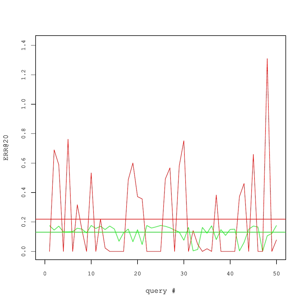
Consider a concrete example of two Information Retrieval (IR) systems, each of which answered 50 queries. The quality of results for each query was measured using a performance metric called the Expected Reciprocal Rank (ERR@20). These numbers are shown in Fig. 1, where average systems' performance values are denoted by horizontal lines.
On average, the red system is better than the green one. Yet, there is high variance. In fact, to produce the Fig. 1, we took query-specific performance scores from one real system and applied an additive zero-centered random noise to generate the other system. If there were sufficiently many queries, this noise would largely cancel out. But for the small set of queries, it is likely that the average performance of two systems would differ.
Fig 1. Performance of two IR systems.
Statistical testing is a standard approach to detect such situations.
Rather than taking average query level values of ERR@20 at their face value, we suppose that there is the sampling uncertainty obfuscating the ground truth about systems' performance. If we make certain assumptions about the nature of randomness (e.g., assume that the noise is normal and i.i.d.), it is possible to determine the likelihood that observed differences are due to chance. In the frequentist inference, this likelihood is represented by a p-value.
The p-value is a probability to obtain an average difference in performance at least as large as the observed one, when truly there is no difference in average systems' performance, or, using the statistical jargon, under the null hypothesis. Under the null hypothesis, a p-value is an instantiation of the uniform random variable between 0 and 1. Suppose that differences in systems' performance corresponding to p-values larger than 0.05 are not considered statistically significant and, thus, ignored. Then, the false positive rate is controlled at 5% level. That is, in only 5% of all cases when the systems are equivalent in the long run, we would erroneously conclude that the systems are different. We would reiterate that in the in frequentist paradigm, the p-value is not necessarily an indicator of how well experimental data support our hypothesis. Measuring p-values (and discarding hypotheses where p-values exceed the 5% threshold) is a method to control the rate of false positives.
Fig. 2. Simulated p-values in 100 experiments, where the true null holds in each experiment.
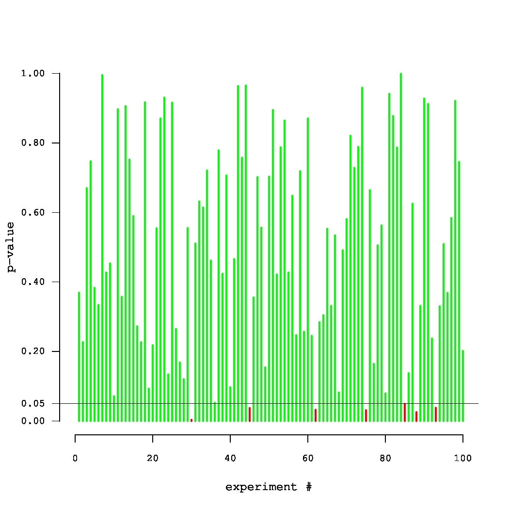
What if the scientist carries out multiple experiments? Consider an example of an unfortunate (but very persistent) researcher, who came up with 100 new systems that were supposed to improve over a given baseline. Yet, they were, in fact, equivalent to the baseline. Thus, each of the 100 p-values can be thought of as an outcome of a uniform random variable between 0 and 1. A set of p-values that could have been obtained in such an experiment is plotted in Fig. 2. The small p-values, below the threshold level of 0.05, are denoted by red bars. Note that one of these p-values is misleadingly small. In truth, there is no improvement in this series of 100 experiments. Thus, there is a danger in paying too much attention to the magnitude of p-values (rather than simply comparing them against a threshold). The issue of multiple testing is universal. In general, most of our hypotheses are false and we expect to observe statistically significant results (all of which are false discoveries) in approximately 5% of all experiments.
This example is well captured by XKCD.
How do we deal with multiple testing? We can decrease the significance threshold or, alternatively, inflate the p-values obtained in the experiments. This process is called an adjustment/correction for multiple testing. The classic correction method is the Bonferroni procedure, where all p-values are multiplied by the number of experiments. Clearly, if the probability of observing a false positive in one experiment is upper bounded by 0.05/100, then the probability that the whole family of 100 experiments contains at least one false positive is upper bounded by 0.05 (due to the union bound).
There are both philosophical and technical aspects of correcting for multiplicity in testing. The philosophical side is controversial. If we adjust p-values in sufficiently many experiments, very few results would be significant! In fact, this observation was verified in the context of TREC experiments (Tague-Sutcliffe, Jean, and James Blustein. 1995, A statistical analysis of the TREC-3 data; Benjamin Carterette, 2012, Multiple testing in statistical analysis of systems-based information retrieval experiments ). But should we really be concerned about joint statistical significance (i.e., significance after we adjust for multiple testing) of our results in the context of the results obtained by other IR researchers? If we have to implement only our own methods, rather than methods created by other people, it is probably sufficient to control the false positive rate only in our own experiments.
We focus on the technical aspects of making adjustments for multiplicity in a single series of experiments. The Bonferroni correction is considered to be overly conservative, especially when there are correlations in data. In an extreme case, if we repeat the same experiment 100 times (i.e., outcomes are perfectly correlated), the Bonferroni correction leads to multiplying each p-value by 100. It is known, however, that we are testing the same method and it is, therefore, sufficient to consider a p-value obtained in (any) single test. The closed testing procedure is a less conservative method that may take correlations into account. It requires testing all possible combinations of hypotheses. This is overly expensive, because the number of combinations is exponential in the number of tested methods. Fortunately, there are approximations to the closed testing procedure, such as the MaxT test, that can also be used.
We carried out an experimental evaluation, which aimed to answer the following questions:
- Is the MaxT a good approximation of the closed testing (in IR experiments)?
- How conservative are multiple comparisons adjustments in the context of a small-scale confirmatory IR experiment?
A description of the experimental setup, including technical details, can be found in our paper (Boytsov, L., Belova, A., Westfall, P. 2013. Deciding on an Adjustment for Multiplicity in IR Experiments. In proceedings of SIGIR 2013.). A brief overview can be found in the presentation slides. Here, we only give a quick summary of results.
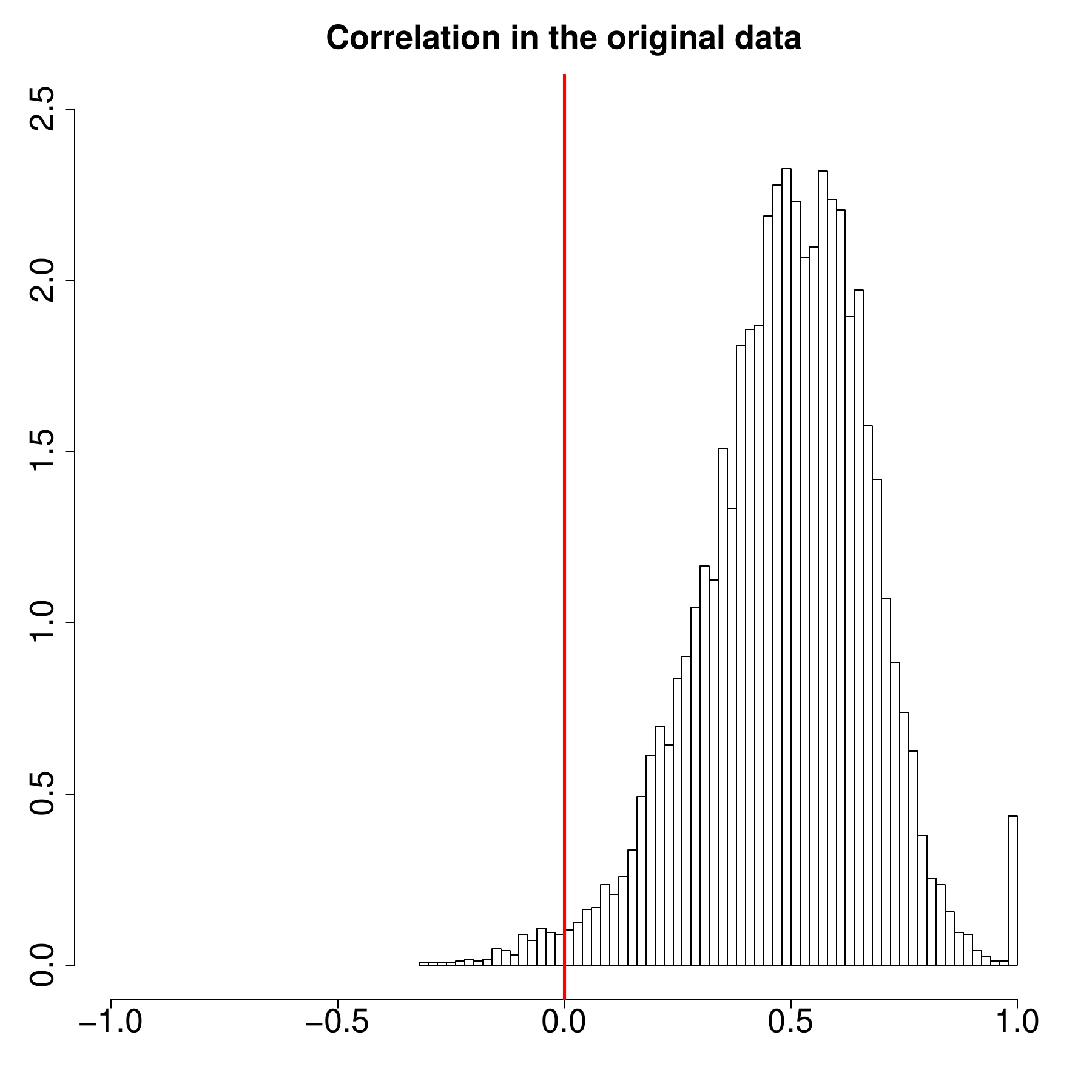
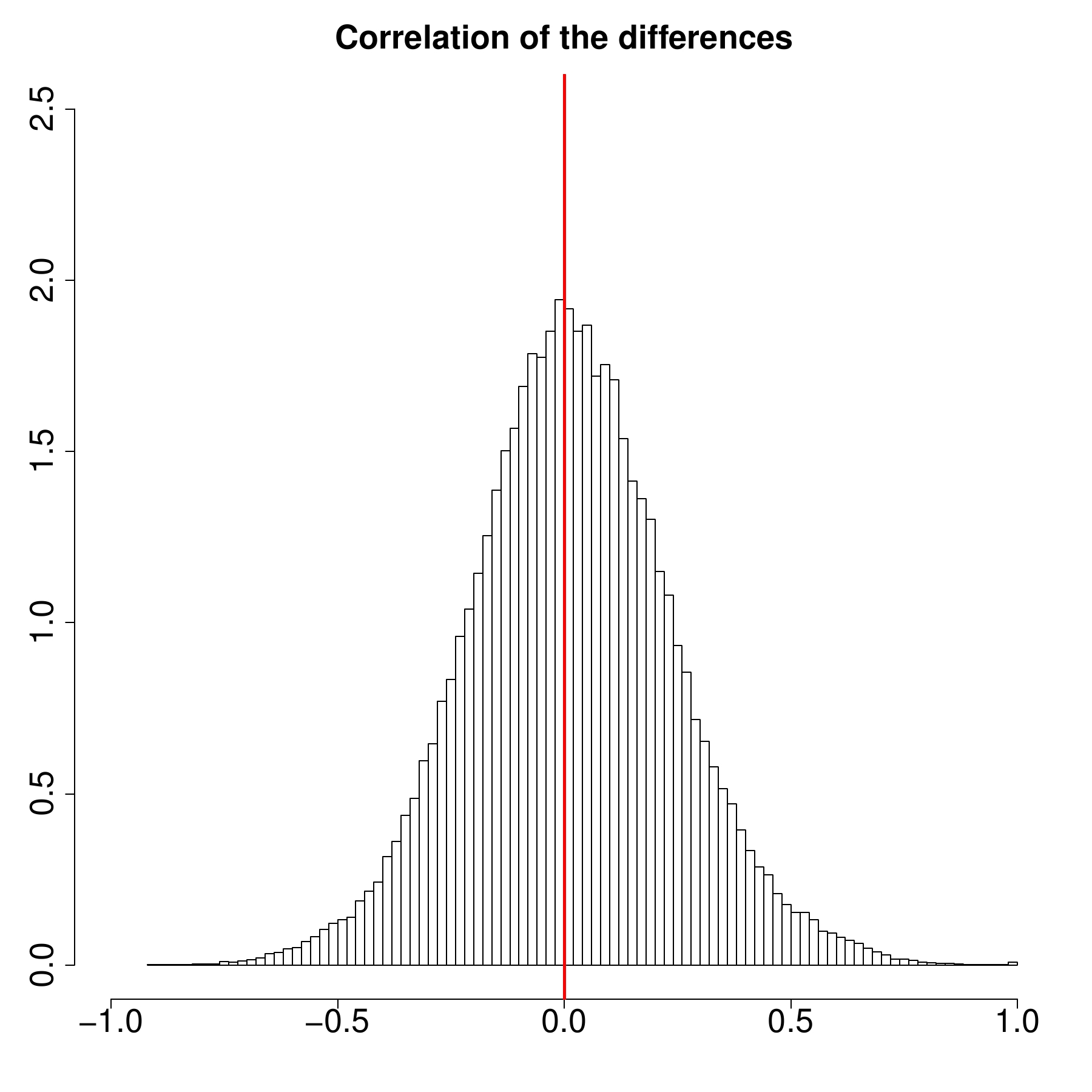
First, in our experiments, the p-values obtained from the MaxT permutation test were almost identical to those obtained from the closed testing procedure. A modification of the Bonferroni adjustment (namely, the Holm-Bonferroni correction) tended to produce larger p-values, but this did not result in the Bonferroni-type correction being much more conservative. This is a puzzling discovery, because performance scores of IR systems (such as ERR@20) substantially correlate with each other (see Fig 3, the panel on the left). In that, both the MaxT permutation test and the closed testing procedure should have outperformed the correlation-agnostic Holm-Bonferroni correction. One possible explanation is that our statistical tests operate essentially on differences in performance scores (rather than scores themselves). It turns out, that there
are fewer strong correlations in performance score differences (see Fig. 3, the panel on the right).
We also carried out a simulation study, in which we measured performance of several systems. Approximately half of our systems were almost identical to the baseline with remaining systems being different. We employed four statistical tests to detect the differences using query sets of different sizes. One of the tests did not involve adjustments for multiplicity. Using average performance values computed for a large set of queries (having 30 thousand elements), we could tell which outcomes of significance testing represented true differences and which were false discoveries. Thus, we were able to compute the number of false positives and false negatives. Note that the fraction of false positives was computed as a fraction of experimental series that contained at least one false positive result. This is called the family-wise error rate.
Table 1. Simulation results for the TREC-like systems. Percentages of false negatives/positives
|
|
|
|
50 |
100 |
400 |
1600 |
6400 |
| Unadjusted test |
85.7/14.4 |
80.8/11.6 |
53.9/10.0 |
25.9/15.4 |
2.5/17.0 |
| Closed test |
92.9/0.0 |
88.8/0.2 |
69.5/1.7 |
36.6/3.1 |
5.2/6.8 |
| MaxT |
93.9/0.0 |
91.8/0.2 |
68.0/1.2 |
35.7/3.0 |
6.3/6.6 |
| Holm-Bonferroni |
94.9/2.0 |
92.5/1.8 |
69.6/2.6 |
37.0/3.2 |
6.5/6.2 |
|
Format: the percentage of false negatives (blue)/false positives (red)
|
|
According to the simulation results in Table 1, if the number of queries is small, the unadjusted test detects around 15% of all true differences (85% false negative rate) . This is twice as many as the number of true differences detected by the tests that adjust p-values for multiple testing. One may conclude that adjustments for multiplicity work poorly and "kill" a lot of significant results. In our opinion, none of the tests performs well, because they discover only a small fraction of all true differences. As the number of queries increases, the differences in the number of detected results between the unadjusted and adjusted tests decrease. For 6400 queries, every test has enough power to detect almost all true differences. Yet, the unadjusted test has a much higher rate of false positives (a higher family-wise error).
Conclusions
We would recommend a wider adoption of adjustments for multiple testing. Detection rates can be good, especially with large query samples. Yet, an important research question is whether we can use correlation structure more effectively.
We make our software available on-line.
Note that it can compute unadjusted p-values as well p-values adjusted for multiple testing. The implementation is efficient (it is written in C++) and accepts data in the form of a performance-score matrix. Thus, it can be applied to other domains, such as classification. We also do provide scripts that can convert the output of TREC evaluation utlities trec_eval and gdeval to the matrix format.
This post was co-authored with Anna Belova
The problem with the previous version of Intel's library benchmark
Submitted by srchvrs on Mon, 04/15/2013 - 01:42
This short post is an update for the previous blog entry. Most likely,
the Intel compiler does not produce the code that is 100x faster, at least, not under normal circumstances. The updated benchmark is posted on the GitHub. Note that the explanation below is just my guess, I will be happy to hear an alternative version.
It looks like the Intel compiler is super-clever and can dynamically adjust accuracy of computation. Consider the following code:
float sum = 0; for (int j = 0; j < rep; ++j) { for (int i = 0; i < N*4; i+=4) { sum += exp(data[i]); sum += exp(data[i+1]); sum += exp(data[i+2]); sum += exp(data[i+3]); } }
Here the sum becomes huge very quickly. Thus, the result of calling exp becomes very small compared to sum. It appears to me that the code built with the Intel compiler does detect this situation. Probably, at run-time. After this happens, the function exp is computed using a very low-accuracy algorithm or not computed at all. As a result, when I ran this benchmark on a pre-historic Intel Core Duo 2GHz, I was still able to crunch billions of exp per second, which was clearly impossible. Consider now the following, updated, benchmark code:
float sum = 0; for (int j = 0; j < rep; ++j) { for (int i = 0; i < N*4; i+=4) { sum += exp(data[i]); sum += exp(data[i+1]); sum += exp(data[i+2]); sum += exp(data[i+3]); } sum /= float(N*4); // Don't allow sum become huge! }
Note line 9. It prevents sum from becoming huge. Now, we are getting more reasonable performance figures. In particular, for single-precision values, i.e., floats,
the Intel compiler produces a code that is only 10x faster compared to code produced by the GNU compiler. It is a large difference, but it is probably due to using SIMD
extensions for Intel.
How fast are our math libraries?
Submitted by srchvrs on Wed, 04/03/2013 - 17:32
The GNU C++ compiler produces efficient code for multiple platforms. The Intel compiler is specialized for Intel processors and produces even more efficient, but Intel-specific code. Yet, as some of us know, one does not get more than 10-20% improvement in most cases by switching from the GNU C++ compiler to the Intel compiler.
(The Intel compiler is free for non-commercial uses.)
There is at least one exception: programs that rely
heavily on a math library. It is not surprising that users of the Intel math library often enjoy almost a two-fold speedup over the GNU C++ library when they explicitly employ highly vectorized, linear algebra, and statistical functions. What is really amazing is that ordinary mathematical functions such as exp, cos, and sin can be computed 5-10 times faster by the Intel math library, apparently, without sacrificing accuracy.
Intel claims a 1-2 order-magnitude speedup for all standard math functions. To confirm this, I wrote simple benchmarks. They run on a modern Core i7 (3.4 GHz) processor in a single thread. The code (available from GitHub) generates random numbers that are used as arguments for various math functions. The intent of this is to represent plausible argument values. Intel also reports performance results for “working” argument intervals and admits that it can be quite expensive to compute functions (e.g., trigonometric) accurately for large argument values.
For single-precision numbers (i.e., floats), the GNU library is capable of computing only 30-100 million mathematical functions per second, while the Intel math library completes 400-1500 million of operations per second. For instance, it can do 600 million exponentiations or 400 million computations of the sine function (with single-precision arguments). This is slower than Intel claims, but still an order of magnitude faster than the GNU library.
Are there any accuracy tradeoffs? The Intel library can work in the high accuracy mode, in which, as Intel claims, the functions should have an error of at most 1 ULP (unit in the last place). Roughly speaking, the computed value may diverge from the exact one only in the last digit of mantissa. For the GNU math library, the errors are known to be as high as 2 ULP (e.g., for the cosine function with a double-precision argument). In the lowest accuracy mode, additional order-of-magnitude speedups are possible. It appears that the Intel math library should be superior to the GNU library in all respects. Note, however, that I did not verify Intel accuracy claims and I appreciate any links in regard to this topic. In my experiments, to ensure that the library works in the high-accuracy mode, I make a special call:
I came across the problem of math-library efficiency, because I needed to perform many exponentiations to integer powers. There is a well-known approach called exponentiation by squaring and I hoped that the GNU math library implemented it efficiently. For example, to raise x to the power of 5, you first compute the square of x using one multiplication, and another multiplication to compute x4 (by squaring x2). Finally, you can multiply x4 by x and return the result. The total number of multiplications is three. Note that the naive algorithm would need four multiplications.
The function pow is overloaded, which means that there are several versions that serve arguments of different types. I wanted to ensure that the correct, i.e., the efficient version was called. Therefore, I told the compiler that the second argument is an unsigned (i.e., non-negative) integer as follows:
Big mistake! For the reason, which I cannot fully understand, this makes both compilers (Intel and GNU) choose an inefficient algorithm. As my benchmark shows (module testpow), it takes a modern Core i7 (3.4 GHz) processor almost 200 CPU cycles to compute x5. This is ridiculously slow, if you take into account that one multiplication can be done in one cycle (or less if we use SSE).
So, the following handcrafted implementation outperforms the standard pow by an order of magnitude (if the second argument is explicitly cast to unsigned):
float PowOptimPosExp0(float Base, unsigned Exp) { if (!Exp) return 1; float res = Base; --Exp; while (Exp) { if (Exp & 1) res *= Base; Base *= Base; Exp >>= 1; }; return res; };
If we remove the explicit cast to unsigned, the code is rather fast even with the GNU math library:
int IntegerDegree=5; pow(x, IntegerDegree);
Yet, my handcrafted function is still 20-50% faster than the GNU pow.
Turns out that it is also faster than the Intel's version. Can we make it even faster? One obvious reason for inefficiency are branches. Modern CPUs are gigantic conveyor belts that split a single operation into a sequence of dozens (if not hundreds) of micro operations. Branches may require the CPU to restart the conveyor, which is costly. In our case, it is beneficial to use only the forward branches. Each forward branch represents a single value of an integer exponent and contains the complete code to compute the function value. This code "knows" the exponent value and, thus, no additional branches are needed:
float PowOptimPosExp1(float Base, unsigned Exp) { if (Exp == 0) return 1; if (Exp == 1) return Base; if (Exp == 2) return Base * Base; if (Exp == 3) return Base * Base * Base; if (Exp == 4) { Base *= Base; return Base * Base; } float res = Base; if (Exp == 5) { Base *= Base; return res * Base * Base; } if (Exp == 6) { Base *= Base; res = Base; Base *= Base; return res * Base; } if (Exp == 7) { Base *= Base; res *= Base; Base *= Base; return res * Base; } if (Exp == 8) { Base *= Base; Base *= Base; Base *= Base; return Base; } … }
As a result, for the degrees 2-16, the Intel library performs 150-250 operations per second, while the customized version is capable of making 600-1200 exponentiations per second.
Acknowledgements: I thank Nathan Kurz and Daniel Lemire for the discussion and valuable links; Anna Belova for editing the entry.
Are regular expressions fast?
Submitted by srchvrs on Fri, 02/15/2013 - 22:59
I was preparing a second post on the history of dynamic programming algorithms, when another topic caught my attention. There is a common belief among developers that regular expression engines in Perl, Java, and several other languages are fast. This has been my belief as well. However, I was dumbfound by a discovery that these engines always rely on a pre-historic backtracking approach (with partial memoization), which can be very slow. In some pathological cases, their run-time is exponential in the length of the text and/or pattern. Non-believers can check out my sample code. What is especially shocking is that efficient algorithms were known already in the 1960s. Yet, most developers were unaware. There are certain cases, when one has to use backtracking, but these cases are rare. For the most part, a text can be matched against a regular expression via a simulation of a non-deterministic or deterministic finite state automaton. If you are familiar with the concept of the finite state automaton, I encourage you to read the whole story here. The other readers may benefit from reading this post to the end.
A finite state automaton is an extremely simple concept, but it is usually presented in a very formal way. Hence, a lot of people fail to understand it well. One can visualize a finite state automaton as a robot moving from floor to floor of a building. Floors represent automaton states. An active state is a floor where the robot is currently located. The movements are not arbitrary: the robot follows commands. Given a command, the robot moves to another floor or remains on the same floor. This movement is not solely defined by the command, but rather by a combination of the command and the current floor. In other words, a command may work differently on each floor.
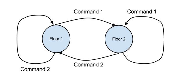
Figure 1. A metaphoric representation of a simple automaton by a robot moving among floors.
Consider a simple example in Figure 1. There are only two floors and two commands understandable by the robot. If the robot is on the first floor, the Command 2 tells the robot to remain on this floor. This is denoted by a looping arrow. However, the Command 1 makes the robot move to the second floor.
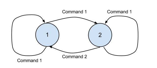
Figure 2. A non-deterministic automaton.
A deterministic robot is very diligent and can only process unambiguous commands. A non-deterministic robot has more freedom and is capable of processing ambiguous commands. Consider an example of a non-deterministic automaton in Figure 2. If the robot is on the first floor and receives Command 1, it may choose to stay on the first floor, or to move to the second floor. Furthermore, there may be floors where robot's behavior is not defined for some of the commands. For example, in Figure 2, if the robot is on the first floor, it does not know where to move on receiving Command 2. In this case, the robot simply got stuck, i.e., the automaton fails.
In the robot-in-the-building metaphor, a building floor is an automaton state and a command is a symbol in some alphabet. The finite state automaton is a useful abstraction, because it allows us to model special text recognizers known as regular expressions. Imagine that a deterministic robot starts from the first floor and follows the commands defined by text symbols. He executes these commands one by one and moves from floor to floor. If all commands are executed and the robot stops on the last floor (the second floor in our example), we say that the automaton recognizes the text. Note that the robot may visit the last floor several times, but what matters is whether it stops on the last floor or not.
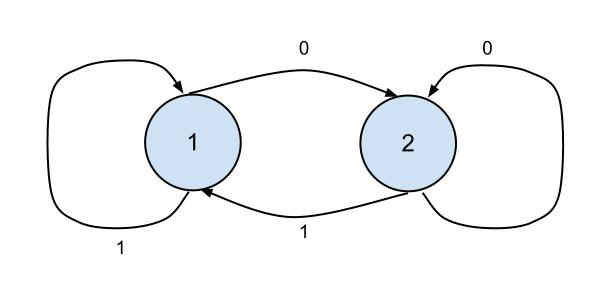
Figure 3. A finite state automaton recognizing binary texts that end with 0.
Consider an example of a deterministic automaton/robot in Figure 3, which works with texts written in the binary alphabet. One can see that the robot recognizes a text if and only if (1) the text is non-empty and (2) the last symbol is zero. Indeed, whenever the robot reads the symbol 1, it either moves to or remains on the first floor. When it reads the symbol 0, it either moves to or remains on the second floor. For example, for the text 010, the robot first follows the command to move to floor two. Then, it reads the next command (symbol 1), which makes it return to floor one. Finally, the robot reads the last command (symbol 0) and moves to the final (second) floor. Thus, the automaton recognizes the string 010. There is a well-known relationship between finite automata and regular expressions. For each regular expression there exists an equivalent automaton and vice versa. For instance, in our case the automaton is defined by the regular expression: 0$.
The robot/automaton in Figure 3 is deterministic. Note, however, that not all regular expressions can be easily modeled using a deterministic robot/automaton. In most cases, a regular expression is best represented by a non-deterministic one. For the deterministic robot, a sequence of symbols/commands fully determines the path (i.e., a sequence of floors) of the robot in the building. As noted previously, if the robot is not deterministic, in certain cases, it may choose several different paths after reading the same command (being also on the same floor). A choice of the path is not arbitrary: some paths are not legitimate (see Figure 2), yet we do not know for sure what is the exact sequence of the floors that the robot will visit. When does the non-deterministic robot recognize the text? The answer is simple: there should be at least one legitimate path that starts on the first and ends on the last floor. If no such path exists, the text is not recognized. From the computational perspective, we need to either find this path or to prove that no such path exists.
A naive approach to find a path that ends on the last floor involves a recursive search. The robot starts from the first floor and reads one symbol/command after another. If the command and the source floor unambiguously define the next floor, the robot simply goes to this floor. Because the robot is not deterministic, there may be more than one target floor sometimes, or no target floors at all. For example, in Figure 2, if the robot is on the first floor and receives the Command 1, it can either move to the second floor or stay on the first floor. However, it cannot process Command 2 on the first floor. If there is more than one target floor, the robot memorizes its state (by creating a checkpoint) and chooses to explore any of the legal target floors recursively. If the robot reaches the place, where no target floors exist, it returns to the last checkpoint and continues to explore (yet unvisited) floors starting from this checkpoint. This method is known as backtracking.
The backtracking approach can be grossly inefficient and may have exponential run-time. A more efficient robot should be able to clone itself and merge together several clones when it is necessary. Whenever the robot has a choice where to move, it clones itself and moves to all possible target floors. However, if several clones meet at the same floor, they merge together. In other words, we have a “Schrodinger” robot that is present on several floors at the same time! Surprisingly enough, this interpretation is often challenged by people, who believe that it does not truly represent the phenomenon of the non-deterministic robot/automaton. Yet, it does and, in fact, this representation is very appealing from the computational perspective. To implement this approach, one should keep a set of floors, where the robot is present. This set of floors corresponds to active states of the non-deterministic automaton. On receiving the next command/symbol, we go over these floors and compute a set of legitimate target floors (where the robot can move to). Then, we simply merge these sets and obtain a new set of active floors (occupied by our Schrodinger robot).
This method was obvious to Ken Thompson in 1960s, but not obvious to the implementers of the backtracking approach in Perl and other languages. I reiterate that classic regular expressions are always equivalent to automata and vice versa. However, there are certain extensions that are not. In particular, regular expressions with backreferences cannot be generally represented by automata. Oftentimes, if a regular expression contains backreferences, the potentially inefficient backtracking approach is the only way to go. However, in most cases regular expressions do not have backreferences, and can be efficiently processed by a simulation of the non-deterministic finite state automaton. The whole process can be made even more efficient through partial or complete determinization.
Edited by Anna Belova
Early life of dynamic programming (Part I)
Submitted by srchvrs on Sat, 12/22/2012 - 20:22
Many software developers and computer scientists are familiar with a concept of dynamic programming. Despite its arcane and intimidating name, dynamic programming is a rather simple technique to solve complex recursively defined problems. It works by reducing a problem to a bunch of overlapping subproblems each of which can be further processed recursively. The existence of overlapping subproblems is what differentiates dynamic programming from other recursive approaches such as divide-and-conquer. An ostensibly drab mathematical issue, dynamic programming has a remarkable history.
The approach originated from discrete-time optimization problems studied by R. Bellman in 1950s and was later extended to a wider range of tasks, not necessarily related to optimization. One classic example is the Fibonacci numbers Fn = Fn-1 + Fn-2. It is straightforward to compute the Fibonacci numbers one by one in the order of increasing n, as well as to memorize the results on the go. In that, computation of Fn-2 is a shared subproblem whose solution is required to obtain both Fn-1 and Fn. Clearly this is just a math trick unrelated to programming. How come was it named so strangely?
There is a dramatic, but likely untrue, explanation given by R. Bellman in his autobiography:
"The 1950s were not good years for mathematical research. We had a very interesting gentleman in Washington named Wilson. He was secretary of Defense, and he actually had a pathological fear and hatred of the word ‘research’. I'm not using the term lightly; I'm using it precisely. His face would suffuse, he would turn red, and he would get violent if people used the term ‘research’ in his presence. You can imagine how he felt, then, about the term ‘mathematical’ … Hence, I felt I had to do something to shield Wilson and the Air Force from the fact that I was really doing mathematics inside the RAND Corporation.
What title, what name, could I choose? In the first place I was interested in planning, in decision making, in thinking. But planning, is not a good word for various reasons. I decided therefore to use the word ‘programming’. I wanted to get across the idea that this was dynamic, this was multistage, this was time-varying—I thought, let’s kill two birds with one stone. Let’s take a word that has an absolutely precise meaning, namely ‘dynamic’, in the classical physical sense … Thus, I thought ‘dynamic programming’ was a good name. It was something not even a Congressman could object to. So I used it as an umbrella for my activities."
(From Stuart Dreyfus, Richard Bellman on the Birth of Dynamic Programming)
This anecdote, though, is easy to disprove. There is published evidence that the term dynamic programming was coined in 1952 (or earlier), whereas Wilson became the secretary of defense in 1953. Wilson held a degree in electrical engineering from Carnegie Mellon. Before 1953, he was a CEO of a major techology company General Motors, while at early stages of his career he supervised development of various electrical equipment. It is, therefore, hard to believe that this man could trully hate the word "research". (The observation on the date mismatch was originally made by Russell & Norvig in their book on artificial intelligence.)
Furthermore, linear programming (which also has programming in its name), appears in the papers of G. Dantzig before 1950. A confusing term "linear programming", as Dantzig explained in his book, was based on the military definition of the word "program", which simply means planning and logistics. In mathematics, this term was adopted to denote optimization problems and gave rise to several names such as integer, convex, and non-linear programming.
It should now be clear that the birth of dynamic programming was far less dramatic: R. Bellman simply picked up the standard terminology and embellished it with the adjective "dynamic", to highlight the temporal nature of the problem. There was nothing unusual in the choice of the word "dynamic" either: The notion of dynamic(al) system (a system with time-dependent states) comes from physics and was widely used already in the 19th century.
Dynamic programming is very important to computational biology and approximate string searching. Both domains use string similarity functions that are variants of the Levenshtein distance. The Levenshtein distance was formally published in 1966 (1965 in Russian). Yet, it took almost 10 years for the community to fully realize how dynamic programming could be used to compute the string similarity functions. This is an interesting story that is covered in a follow-up post.
Edited by Anna Belova
Pages

|
|
 |
|
|
 |
 |
 |
|
|
|